%----->>>>VOLUME 1, NUMBER 2 OF SOLSTICE. WINTER, 1990; 10:07 PM
12/12/90.
 %----->>>>HAPPY HOLIDAYS!!!! Sandy Arlinghaus.
 %----->>>>IF YOU DO not WISH TO CONTINUE YOUR COMPLIMENTARY SUBSCRIPTION,
 %----->>>>FOR 1991, PLEASE WRITE Solstice@UMICHUM AND SO INDICATE.
 %----->>>>THANK YOU FOR PARTICIPATING IN GEOGRAPHY'S FIRST E-JOURNAL.
 %----->>>>HARD-COPY OF VOLUME I IS AVAILABLE AS MONOGRAPH 13 IN THE
 %         IMaGe MONOGRAPH SERIES.
 \hsize = 6.5 true in %THIS FILE CONTAINS TYPESETTING CODE, ONLY.
  %ADD IT TO THE BEGINNING OF EACH OF THE FOLLOWING FILES TO TYPESET THEM.
  %ALSO ADD \bye TO CLOSE EACH FILE TO BE TYPESET.
 \input fontmac %delete to download, except on Univ. Mich. (MTS) equipment.
 \setpointsize{12}{9}{8}%same as previous line; set font for 12 point type.
 \parskip=3pt
 \baselineskip=14 pt
 \mathsurround=1pt
 \headline = {\ifnum\pageno=1 \hfil \else {\ifodd\pageno\righthead
   \else\lefthead\fi}\fi}
 \def\righthead{\sl\hfil SOLSTICE }
 \def\lefthead{\sl Winter, 1990 \hfil}
 \def\ref{\noindent\hang}
 \font\big = cmbx17
 \font\tn = cmr10
 \font\nn = cmr9 %The code has been kept simple to facilitate reading as
e-mail
 \font\tbf = cmbx12
 \outer\def\heading#1\par{\vskip 0pt plus .1\vsize \penalty-50
   \vskip 0pt plus -.1\vsize \medskip\vskip\parskip
   \centerline{\tbf#1}\nobreak\medskip\noindent}
 \outer\def\section#1\par{\vskip 0pt plus .1\vsize \penalty-50
   \vskip 0pt plus -.1\vsize \medskip\vskip\parskip
   \leftline{\tbf#1}\nobreak\smallskip\noindent}
 \outer\def\subsection#1\par{\vskip 0pt plus .1\vsize \penalty-50
   \vskip 0pt plus -.1\vsize \medskip\vskip\parskip
   \leftline{\sl#1}\nobreak\smallskip\noindent}

 \def\pmb#1{\setbox0=\hbox{#1}%
     \kern-.025em\copy0\kern-\wd0
     \kern.05em\copy0\kern-\wd0
     \kern-.025em\raise.0433em\box0 }

 \centerline{\big SOLSTICE:}
 \vskip.5cm
 \centerline{\bf  AN ELECTRONIC JOURNAL OF GEOGRAPHY AND MATHEMATICS}
 \vskip5cm
 \centerline{\bf WINTER, 1990}
 \vskip12cm
 \centerline{\bf Volume I, Number 2}
 \smallskip
 \centerline{\bf Institute of Mathematical Geography}
 \vskip.1cm
 \centerline{\bf Ann Arbor, Michigan}
 \vfill\eject
 \hrule
 \smallskip
 \centerline{\bf SOLSTICE}
 \line{Founding Editor--in--Chief:  {\bf Sandra Lach Arlinghaus}. \hfil}
 \smallskip
 \centerline{\bf EDITORIAL BOARD}
 \smallskip
 \line{{\bf Geography} \hfil}
 \line{{\bf Michael Goodchild}, University of California, Santa Barbara.
\hfil}
 \line{{\bf Daniel A. Griffith}, Syracuse University. \hfil}
 \line{{\bf Jonathan D. Mayer}, University of Washington; joint appointment
  in School of Medicine.\hfil}
 \line{{\bf John D. Nystuen}, University of Michigan (College of
  Architecture and Urban Planning).}
 \smallskip
 \line{{\bf Mathematics} \hfil}
 \line{{\bf William C. Arlinghaus}, Lawrence Technological University. \hfil}
 \line{{\bf Neal Brand}, University of North Texas. \hfil}
 \line{{\bf Kenneth H. Rosen}, A. T. \& T. Information Systems Laboratory.
        \hfil}
 \smallskip
 \line{{\bf Business} \hfil}
 \line{{\bf Robert F. Austin},
 Director, Automated Mapping and Facilities Management, CDI. \hfil}
 \smallskip
 \hrule
 \smallskip

       The purpose of {\sl Solstice\/} is to promote  interaction
 between geography and mathematics.   Articles in which  elements
 of   one  discipline  are used to shed light on  the  other  are
 particularly sought.   Also welcome,  are original contributions
 that are purely geographical or purely mathematical.   These may
 be  prefaced  (by editor or author) with  commentary  suggesting
 directions  that  might  lead toward  the  desired  interaction.
 Individuals  wishing to submit articles,  either short or full--
 length,  as well as contributions for regular  features,  should
 send  them,  in triplicate,  directly to the  Editor--in--Chief.
 Contributed  articles  will  be refereed by  geographers  and/or
 mathematicians.   Invited articles will be screened by  suitable
 members of the editorial board.  IMaGe is open to having authors
 suggest, and furnish material for, new regular features.
 \vskip2in
 \noindent {\bf Send all correspondence to:}
 \vskip.1cm
 \centerline{\bf Institute of Mathematical Geography}
 \centerline{\bf 2790 Briarcliff}
 \centerline{\bf Ann Arbor, MI 48105-1429}
 \vskip.1cm
 \centerline{\bf (313) 761-1231}
 \centerline{\bf IMaGe@UMICHUM}
 \vfill\eject

       This  document is produced using the typesetting  program,
 {\TeX},  of Donald Knuth and the American Mathematical  Society.
 Notation  in  the electronic file is in accordance with that  of
 Knuth's   {\sl The {\TeX}book}.   The program is downloaded  for
 hard copy for on The University of Michigan's Xerox 9700 laser--
 printing  Xerox machine,  using IMaGe's commercial account  with
 that University.

 Unless otherwise noted, all regular features are written by the
 Editor--in--Chief.
 \smallskip
       {\nn  Upon final acceptance,  authors will work with IMaGe
 to    get  manuscripts   into  a  format  well--suited  to   the
 requirements   of {\sl Solstice\/}.  Typically,  this would mean
 that  authors    would  submit    a  clean  ASCII  file  of  the
 manuscript,  as well as   hard copy,  figures,  and so forth (in
 camera--ready form).     Depending on the nature of the document
 and   on   the  changing    technology  used  to  produce   {\sl
 Solstice\/},   there  may  be  other    requirements  as   well.
 Currently,  the  text  is typeset using   {\TeX};  in that  way,
 mathematical formul{\ae} can be transmitted   as ASCII files and
 downloaded   faithfully   and   printed   out.    The     reader
 inexperienced  in the use of {\TeX} should note that  this    is
 not  a ``what--you--see--is--what--you--get"  display;  however,
 we  hope  that  such readers find {\TeX} easier to  learn  after
 exposure to {\sl Solstice\/}'s e-files written using {\TeX}!}

       {\nn  Copyright  will  be taken out in  the  name  of  the
 Institute of Mathematical Geography, and authors are required to
 transfer  copyright  to  IMaGe as a  condition  of  publication.
 There are no page charges; authors will be given  permission  to
 make reprints from the electronic file,  or to have IMaGe make a
 single master reprint for a nominal fee dependent on  manuscript
 length.   Hard  copy of {\sl Solstice\/}  will be sold  (contact
 IMaGe  for  price--{\sl Solstice\/} and will be priced to  cover
 expenses  of journal production);  it is the desire of IMaGe  to
 offer  electronic  copies to  interested parties for free--as  a
 kind of academic newsstand at which one might browse,  prior  to
 making purchasing decisions.  Whether or not it will be feasible
 to  continue distributing complimentary electronic files remains
 to be seen.}
 \vskip.5cm
 Copyright, December, 1990, Institute of Mathematical Geography.
 All rights reserved.
 \vskip1cm
 ISBN: 1-877751-44-8
 \vfill\eject
 \centerline{\bf SUMMARY OF CONTENT}
 \smallskip
      Numbering  given  below  corresponds  to the number  of the
 electronically transmitted file.
 \smallskip
 \noindent 1.  Typesetting code; file of {\TeX} commands that may
 be inserted at the beginning of each file  (or in front  of  the
 whole set run at once) in order to typeset the document.
 \smallskip
 \noindent 2.  File of front matter, including this material!
 \smallskip
 \noindent 3 and 4.  Reprint of John D. Nystuen from 1974.
 {\sl A city of strangers:   Spatial aspects of alienation in the
 Detroit metropolitan region.}
 \smallskip

    Examines urban shift from ``people space" to ``machine space"
 (see R. Horvath, {\sl Geographical Review\/} April, 1974) in the
 context  of  the  Detroit  metropolitan region of 1974.  As with
 Clifford's {\sl Postulates of the Science of Space\/}, reprinted
 in the last issue of {\sl Solstice\/}, note the  timely  quality
 of many of the observations.
 \smallskip
 \noindent 5.  Sandra Lach Arlinghaus.  {\sl Scale and dimension:
 Their logical harmony\/}
 \smallskip

      Linkage between scale  and  dimension  is  made  using  the
 Fallacy of Division and the Fallacy of Composition in a  fractal
 setting.
 \smallskip
 \noindent 6 and 7.  Sandra Lach Arlinghaus.
 {\sl  Parallels  between parallels.\/}  A manuscript  originally
 accepted  by  the  now--defunct  interdisciplinary  journal,
 {\sl Symmetry}.
 \smallskip

      The earth's sun introduces a symmetry in  the  perception  of
 its trajectory in the sky that naturally  partitions  the  earth's
 surface into zones of affine and hyperbolic geometry.  The  affine
 zones, with single geometric  parallels,  are  located  north  and
 south of the geographic tropical parallels.  The hyperbolic  zone,
 with  multiple  geometric  parallels,  is  located   between   the
 geographic  tropical  parallels.   Evidence  of   this   geometric
 partition is  suggested in  the  geographic  environment---in  the
 design of houses and of gameboards.
 \smallskip
 \noindent 8.   Sandra L. Arlinghaus,  William C. Arlinghaus,  and
 John D. Nystuen. {\sl The Hedetniemi  matrix  sum:  A real--world
 application.\/}
 \smallskip

 In  a  recent paper,  we presented an algorithm for  finding  the
 shortest distance between any two nodes in a network of $n$ nodes
 when  given only distances between  adjacent  nodes  [Arlinghaus,
 Arlinghaus,  Nystuen,  {\sl  Geographical Analysis, 1990\/}].  In
 that  previous  research,    we  applied  the  algorithm  to  the
 generalized  road network graph surrounding  San  Francisco  Bay.
 Here, we examine consequent changes  in  matrix  entries when the
 underlying adjacency pattern of  the road  network was altered by
 the 1989 earthquake that closed  the  San Francisco--Oakland  Bay
 Bridge.
 \smallskip
 \noindent 9.  Sandra Lach Arlinghaus.
 {\sl Fractal geometry of infinite pixel sequences:
 ``Super--definition" resolution?}
 \smallskip

 Comparison of space--filling qualities of square and hexagonal
 pixels.
 \smallskip
 \noindent 10.  {\sl Construction Zone\/}.  Feigenbaum's number;
 a triangular coordinatization of the Euclidean plane.
 \vfill\eject
 \centerline{\bf INDUSTRIAL WASTELAND RIVER}
 \centerline{\bf Photograph by John D. Nystuen; Rouge River, Detroit, 1974.}
 \centerline{\bf FRONTISPIECE:  A City of Strangers.}

Click here for Frontispiece
 \vfill\eject
 \centerline{\bf A CITY OF STRANGERS:}
 \centerline{\bf SPATIAL ASPECTS OF ALIENATION IN}
 \centerline{\bf THE DETROIT METROPOLITAN REGION.}
 \smallskip
 \centerline{\sl John D. Nystuen}
 \centerline{The University of Michigan, Ann Arbor}
 \smallskip
 \centerline{An invited address given in the conference:}
 \centerline{\it Detroit Metropolitan Politics:  Decisions and Decision
Makers}
 \centerline{Conference held at Henry Ford Community College}
 \centerline{April 29, 1974}
 \centerline{Dearborn, Michigan}
 \centerline{Comments added, 1990}

      Suburbanization  at the edge of the metropolitan region  and
 the  destruction  of  homes in the  inner  city  through  ``urban
 renewal''   or   expressway  construction  are  the  results   of
 uncoordinated  and decentralized decisions made by people  remote
 from those directly affected.   Unwanted  transportation  burdens
 are  forced  on us by changes in the  location of population  and
 jobs.   There has been a shift,  still continuing,  from ``people
 space'' to ``machine  space'' [5] in our  cities  which  we  seem
 powerless to stem.  ``Machine spaces'' are those spaces dedicated
 to machines or to inter--regional facilities which present larger
 than human, impersonal and often hostile, aspects of society.  We
 are  alienated  from our urban environment to the degree  it  has
 become machine space.   We are alienated from land controlled  by
 strangers.    These   strangers   may  be  decision   makers   in
 institutions   with  metropolitan--wide  jurisdictions  such   as
 transportation planning authorities,  mortgage and banking firms,
 and the regional power company.  The  interests of people of this
 type  are  at least focused on the  metropolis.   Other  decision
 makers affecting local land use are outlanders whose concerns are
 not  exclusively  local.   One type of outlander is the  decision
 maker at state and federal level,  concerned with and responsible
 for general policy of some aspect of urban life but whose  vision
 cannot   be   expected  to  distinguish  variations   in    every
 neighborhood within his/her broad jurisdiction.  Other outlanders
 are decision makers in multi--state or international corporations
 and institutions whose structures extend horizontally across many
 communities   or   even  continents.    Their   aspirations   and
 understanding  of urban life are often incommensurate with  local
 community objectives.  Misunderstanding, alienation, and conflict
 easily result.

 \heading {The Cost of Victory over the ``Tyranny of Space"}

      From the geographical point of view these disturbing aspects
 or  urban  life  today  are the result of our  victory  over  the
 ``tyranny  of space [7]."  Much of the technological  achievement
 of  our  society  has  been  improvement  in  transportation  and
 communication.   We made the oceans routes not barriers; achieved
 air  and  space flight;  built power transmission lines  to  move
 energy,  and  sewer lines to carry off  wastes.   Innovations  in
 communication  are  equally  important.   The  invention  of  the
 alphabet  was  a  great  achievement in  ancient  times  (history
 begins);   the   printing  press  followed  in   medieval   times
 (information  widely shared);  today we have mini--computers made
 of  inexpensive  printed circuits.   Electronic  data  processing
 (embracing  complexity) is as revolutionary as the  alphabet  and
 the  printing press.  The change which will be forthcoming can be
 only  dimly  perceived.   These  inventions  affect  society   by
 radically  changing  spatial and temporal limits within which  we
 are  confined.   This freedom over space and linear  time,  while
 closely  linked  to  the rise in  our  standard  of  living,  now
 threatens  us  in  other  ways.    Previously,   local  community
 organization  and control processes developed relatively free  of
 outside   interference  because  of  the  friction  of  distance.
 Decisions  about  local land uses and activities had to  be  made
 locally  because  control  at a  distance  was  too  inefficient.
 Freedom  from  the tyranny of space has made us subject to  other
 tyrannies  which may be worse.   The opportunity to control at  a
 distance  which technology offers us may be seized by  those  who
 are  indifferent  to others' needs,  selfish and unscrupulous  in
 their quest for power.  Too often one man's gain is another man's
 loss.  The unscrupulous become anonymous and unreachable by being
 hidden in vast institutional hierarchies.  Traditional mechanisms
 of  social  control and the means to draw people to act  for  the
 good of the community are lost.  The community is lost in the old
 geographical  sense.  We  are  a city of  strangers.   I  do  not
 advocate  giving  up our  victory over space.   Instead  we  must
 consider new means of association and control that will  humanize
 the space around us once again.

 \heading Alienated Space

      Alienated land in the sense I am using it has two  meanings.
 It  is  any place where humans are not welcome or may be in  real
 danger;  lands dedicated to machines are of this type.  But it is
 also space controlled by strangers,  perhaps pleasant places from
 which we are excluded by fences and ``no trespassing'' signs,  or
 places  we may enjoy but over which we have no control as to  how
 they  are   to be used or changed;  state and federal  parks  are
 examples.   We  may  find ourselves excluded  from  many  places,
 subject  to regulations in others and even in that  kingdom,  our
 own  home,  denied the right to modify it as we see  fit.  Little
 wonder  we  feel a certain detachment and alienation.    Loss  of
 sense of community is the price for our victory over the  tyranny
 of space.  Machine space and control of community or neighborhood
 by strangers are the consequences.

 \heading {Machine space}

       Ron  Horvath,  in  an  article  in  the  {\sl  Geographical
 Review\/} entitled ``Machine Space,'' classified land parcels  as
 ``machine  space''   rather than ``people space'' depending  upon
 ``who  or  what  is  given priority of use  in  the  event  of  a
 conflict'' [Horvath,  p.  169].   He then pointed out how much of
 our  cities  we  have  given  up  to  machines,   especially  the
 automobile.  He characterized this machine as the  ``sacred cow''
 in American culture.  He said

 {\narrower{ \noindent
 In the minds of many Westerners,  India's sacred cow has come to
 symbolize  the  lengths  to which people will go  to  preserve  a
 nonfunctional   cultural  trait.    But  India's  sacred  cow  is
 downright  rational  in  comparison to  ours.   Could  an  Indian
 imagine devoting 70 percent of downtown  Delhi to cow trails  and
 pasturage as we do for our automobiles in Detroit and Los Angeles.
 Every year nationally we sacrifice more than 50,000 Americans  to
 our sacred cow in traffic accident fatalities (Figure 1)
 [2, p. 168].\par}}

 \topinsert \vskip11cm
 \noindent {\bf Figure 1.}
 ``Machine Space'' in downtown Detroit, ground level, 1971, by R.
 Horvath.  Map reprinted with permission of The American
 Geographical Society, from ``Machine Space," R. Horvath, {\sl The
 Geographical Review\/}, April, 1974, p. 171.
Click here for Figure
1.
\endinsert
  \noindent   Something  like  20 percent of  our  gross  national
 product is tied directly to manufacturing,  servicing and fueling
 the  automobile---twice  the  amount we spend  on  war  machines,
 another  more  sinister genre of sacred cow machine to  which  we
 seem addicted.

 \heading {Vertical Control or Scale Transforms.}

      There  are  signs  of a reaction setting  in.   Ralph  Nader
 effectively  pointed  out that automobiles are  ``unsafe  at  any
 speed."  The solution called for is not crash proof cars.   It is
 reduction  of  exposure by reducing passenger miles  traveled  by
 private automobiles.   We can accomplish this in two very general
 ways:    by  developing mass transit systems and by reducing  the
 number  and  length  of trips taken.  The latter calls  for  re--
 ordering  land use patterns or changing our life style by  giving
 up  some  of  our triumphs over space.   Trends  in  the  Detroit
 Metropolitan Area suggest otherwise.  We are still in the process
 of  completing an expressway system.   The state  has  authorized
 one--half  cent  of the nine cent gasoline tax to be  devoted  to
 mass transit systems;  a significant step but hardly a major re--
 allocation  of  priorities.    SEMTA,  the  state  transportation
 authority for Southeast Michigan,  has recently released its mass
 transportation  plan calling for a 1990 completion date.   If the
 experience  of systems such as the San Francisco Bay Area's  BART
 can  be  taken  as an example,  significant  delays  due  to  the
 operation  of political processes will set that date further into
 the future, if indeed, the system is ever built.
 [As of 1990,  the Southeastern Michigan Transportation  Authority
 (SEMTA)  is defunct.  Their mass transit plan,  released in 1975,
 called for a 1990 completion date  (Figure 2).   All that came of
 this  plan  was  the  elevated  downtown  Detroit  People  Mover,
 delayed,  over  budget,  and out--of--control as the rest of  the
 mass  transportation plan was never implemented and doomed to  go
 out of business.  Too massive to tear down without great expense,
 it  will  remain a bizarre monument to  inadequate  planning  and
 fragmented  action.   On the other hand,  the Detroit  expressway
 system is largely completed.  A final link in the circumferential
 network,  I-696,  opened in 1989, twenty--five years after it was
 proposed.   This  stretch  of expressway was met with  determined
 opposition  from an upper--middle  class,  politically  effective
 neighborhood.   The final links were modified to lessen impact on
 adjacent   residents.    Neighborhoods  near  downtown  locations
 succumbed  to  the  huge  concrete  corridors  years  ago.    The
 expressways created huge barriers and the livable spaces  between
 them proved too fragmented to sustain and are now abandoned.]
 \topinsert \vskip20cm
 \noindent {\bf Figure 2.}  Map from 1974 suggests a network that
 was never built (as of 1990).
Click here for Figure 2.
 \endinsert

 Multi--million dollar transportation projects greatly affect land
 use patterns and are once--and--for--all investments.   They come
 infrequently  and permanently affect the geography of the region.
 The massive water and interceptor plan of the Detroit Water Board
 is  a similar large scale project with more benign  consequences.
 This  brought water from Lake Huron via tunnel and aqueduct to  a
 large  portion  of  the metropolitan  region.   [It  was  also  a
 planning error.  In retrospect we see it was overbuilt due to the
 decline in heavy industry in the city and the exodus of people to
 the suburbs.]

 Decisions  associated with large scale projects are  examples  of
 factors  which  are out of the hands of the ordinary  citizen  or
 even  the  large  land developers working in  the  region.   They
 impose important constraints on land use possibilities.  They are
 decisions  made by strangers and represent a loss of  private  or
 small  community  freedom  of choice.   Many gross forms  in  the
 Detroit metropolitan region are the consequence of decisions made
 many decades ago.  Some individuals and communities try to resist
 the pressures of single large scale commitments.   In the case of
 water procurement,  this can be done by using local ground  water
 wells and septic tanks or small municipal sewage plants.   At low
 population  densities  these  local devices may work fine  and  a
 decentralized  system  is  probably  best.   At  high  densities,
 however,  local  environmental capacities  are  exceeded.   Other
 public agencies,  such as the County Health Departments, may then
 operate  to pressure communities into the larger system.   It  is
 this  hierarchical ordering of systems that removes local control
 from  one aspect after another of urban life.  When  the  problem
 condition   in  the  environment  enlarges  previously   separate
 problems begin to merge,  the best institutional response we have
 yet  devised  is  to establish a  hierarchically  ordered  social
 process to address the larger problem.   This change in scale may
 result  in  qualitatively  different  situations.    Institutions
 operating  at metropolitan levels may appear very inflexible  and
 arbitrary    from  the  point  of  view  of  a  local  authority,
 municipality,    or   private   home   owner.    The   need   for
 standardization and routinization is absolutely crucial for  such
 organizations.   Alienation  may develop between parties who view
 things at different scales without anyone being at fault.

 Politically, a metropolitan region is hierarchically organized by
 spatial  jurisdictions.   Local problems are  most  appropriately
 dealt  with by local authority and regional problems by  regional
 authorities.   We  have  yet  to  devise a  means  of  graciously
 transferring jurisdiction up or down the hierarchy to  correspond
 to  changes in scale in the nature of the problems.   Our greatly
 increased  capacity to overcome transportation and  communication
 costs has led to changes in  population density and locations  of
 jobs which have often exacerbated local problems and called forth
 a scale transfer.  The local community, no longer able to perform
 the  service,  loses  jurisdiction  over the problem   to  higher
 authorities.   At a higher level, much of the loss of state power
 to  the federal government has been a change of  this  sort.  [To
 some  extent  deregulation efforts of recent years prior to  1990
 have shifted responsibility back to local authorities, especially
 from  Federal to State levels.   Hierarchies need to be  designed
 that   set limits or levels of acceptable performance but  remain
 tolerant  of variation in local actions.   State rules  regarding
 equalization   of   county  property  taxes  and   local   school
 performance are examples.]

 \heading {Horizontal Control.}

 Some  institutions  and corporations are cross--threaded  in  the
 fabric  of  society.   Their interests and actions are  uncoupled
 from the local community because they are interested in a  single
 category  of  phenomena  and  not  in  the  mix  of  all  spatial
 categories  at  one  location.   The  decision  makers  in  these
 organizations  are very likely to be outlanders;  people who live
 in  entirely  different communities or even  other  nations,  yet
 whose decisions may be controlling factors in a  local situation.
 The ability of multi--plant firms to make long distance decisions
 is  closely tied to the effectiveness of channels of control  via
 communication  and transportation facilities.   As  communication
 improves  the management has the option to  centralize   decision
 making,  thereby reducing the autonomy of each plant manager.  In
 times   of   poorer  communication  major   decisions   regarding
 enlargement  or  closing  of plants would have been made  at  the
 headquarters of the central management.  A local community  finds
 its fortunes very much in the hands of outlanders.   Three subtle
 and disturbing aspects may characterize such a relationship.   In
 the  first  place  the  central management may  act  in  what  it
 believes  to  be  rational and moral purposes  in  closing  least
 profitable  facilities  in  favor of expansion  in   areas  which
 promise higher returns.  The overall result may be pernicious.  A
 supermarket  chain operating under such rules may end up  closing
 all  its  stores in the inner city in favor of  suburban  stores.
 The  internal  firm reasons may make complete  sense;  close  the
 oldest  facilities  on lots too small to accommodate  the  latest
 technologies,  in  neighborhoods which have declining populations
 and which do not yield high returns because of general low income
 levels.   Inner city neighborhoods with older retired people  and
 poverty  stricken  ethnic  groups,  losing  population  to  urban
 renewal  or  expressway  construction end up losing  their  local
 supermarket.   They are the least able to afford the loss.    The
 decision  may be made in another city by outlanders  unresponsive
 to  the  local  peoples' problems and with no  court  of  appeals
 available.

 A second difficulty for the local community with a plant owned by
 an  international corporation is the policy of the corporation to
 keep its young and most talented management moving from place  to
 place in order that they can learn the business and eventually be
 able to assume roles higher up in the corporate hierarchy.  It is
 a   perfectly reasonable policy with respect to the internal firm
 requirements.   The consequence,  however, is a cadre of talented
 nomads who show little or no interest in the local welfare of the
 community in which they are temporarily located.   Nor would  the
 community  want  to commit political resources to such people  if
 they expressed an interest.   They are simply removed from making
 a  local  community  contribution which they  might  easily  have
 pursued  had they been permanently in the  community.   The  only
 loyalty  that  makes sense to them is  company  loyalty.   Higher
 corporate management is certainly not going to  discourage this.
  A  third  tendency  of  horizontal  cross--community  control  in
 society  is  the homogeneity of facilities  and  company  policy.
 Hierarchies   work  best  under  standard  operating  procedures.
 Economies  of scale are possible,  substitution of  material  and
 personnel  from  one locality to another are facilitated  if  the
 installations  are all the same.   If disciplined standardization
 and  routinization  has  been enforced top  management  can  make
 broad,  basic  decisions secure in the knowledge  that  countless
 local  exceptions  will  not  subvert  their  intent  during  the
 implementation  phase.   But  what happens when accommodation  to
 local  situations  is required.   You may get a  machine  answer,
 ``that  request  will  not compute!'' or more  likely  the  local
 manager  will say,  ``I sure would like to help you but my  hands
 are  tied  by company policy." He may not be telling  the  truth.
 The  impersonal  corporate  presence is an easy way  to  solve  a
 problem by defining oneself out of any concern or responsibility.
 Of  course,  he may be telling the truth but be as  powerless  to
 change corporate policy as the outsider seeking accommodation.

 \heading {We Are the Enemy}

 Pogo said, ``We have met the enemy, and he is us'' [Kelly, 1972].
 All   metropolitan areas are complex.   The Detroit region is  no
 exception.  There  is no one to blame for the mess.   We are  the
 enemy;  we are the city of strangers.   There is no single leader
 or group,  either evil or benign to blame.   The land use pattern
 grows from our decentralized decision processes.   The  decisions
 which  actually affect local land use extend over time and  space
 well beyond the here and now.  It is true the channels of control
 could  be in the hands of evil doers and we could improve our lot
 by exposing and removing them.  But I  think we are not generally
 in  the hands of the unscrupulous;  not even in the hands of  the
 stupid and insensitive.  It just appears that way.  Each decision
 or  action  is  contingent upon conditions that  are  beyond  the
 control  of the individual or group making a  particular  choice.
 There  is  rarely  an instance where these  constraints  are  not
 present.   The  outcome  often  seems  stupid  or  callous.  Most
 deleterious  outcomes  are  probably  unanticipated.    They  are
 indirect effects not thought of by the decision makers.   We need
 to  understand our urban processes well enough to take action  to
 avoid  effects  which  cause discomfort or  inequity  to  others.
 Constraints on decisions may be classed into three groups.  There
 are  institutional  and legal policies.  There are  physical  and
 natural  environmental limitations which have to do with laws  of
 nature  and  the  technological  capacities  with  which  we  may
 accommodate to those laws.  And finally, there are limitations to
 our aspirations and goals,  the imagined conditions that motivate
 our   actions.    These  aspirations  are  not  hampered  by  any
 finiteness of imagination in any single pursuit,  for we all know
 flights  of  imagination  are  boundless.  Rather  limits  appear
 because we harbor multiple needs which are often in conflict.  We
 choose  to  restrain our objectives in one pursuit  in  order  to
 achieve goals in other pursuits.   For example we find it hard to
 have large lots and big lawns which provide us with seclusion and
 status  and  at  the  same  time have  many  close  and  friendly
 neighbors  which make available to us the pleasures and  security
 of sharing a close community.   Under most circumstances to  gain
 one value is to lose the other.

 \heading {Scale Attributes of Value Systems}

 A  definition of values is that they are an individual's feelings
 about   and  identification  with  things  and  people   in   his
 environment.   Values have scale attributes.   Another three fold
 classification is convenient.  There are {\it individual/familial
 identification\/},  a  commitment to proxemic space --- the space
 within  which one touches,  tastes and smells  things.   Secondly
 there   is  {\it  community  identification\/},   embracing   the
 individual's  feelings and concern for those with whom he or  she
 lives and interacts,  not in the same house,  but in the vicinity
 or  neighborhood.  This is local space generally recognizable  by
 sight  and  smell.  Finally  there  is  {\it  political--cultural
 identification\/}  which refers to ideals and concerns  extending
 beyond  the people and community with which the person has  daily
 contact.   This  realm must be dealt with abstractly and  through
 instruments,  either  mechanical or institutional for it  is  too
 large to be perceived by the  senses directly.   This is national
 or global space.   Machine space and control by outlanders may be
 viewed  as  intrusions into our community space by  organizations
 and facilities of this  larger domain.   How they look,  sound or
 smell  has  not  been taken into account in the  design  of  such
 facilities.   Examples include Edison power stations,  the  Lodge
 and Ford expressways, and Detroit  Metropolitan Airport.  We give
 up local community values for the benefits of the global mobility
 and interaction.   Metropolitan life pushes us to scale extremes.
 We   value   individual  rights  and  perogatives  and   mainline
 connections  with the global culture over familial and  community
 concerns.  Intermediate  spatial  scale  values  suffer  and  the
 community declines along with them.   The consequences are visual
 blight,   noise  pollution,   reduced  security,  and  injustice.
 Community values include concern for our fellow man,  a sense  of
 equity  and humaneness.  The mechanisms for enforcing a community
 code  of  ethics are ostracism,  social pressure and the  use  of
 sense  of  humor  to keep people responding to  others  as  human
 beings.   These   mechanisms  do  not  work well  in  a  city  of
 strangers   and  are  not  followed.    They   are   particularly
 ineffective in those large impersonal machine spaces, the streets
 and  expressways,   bus  stations,  terminals and  warehouse  and
 factory  districts.  The urban code of ethics carefully preserves
 the  privacy of individuals and tolerates eccentrics.   A  person
 has  functional but fragmented value and is valued  for  specific
 tasks he or she can do.   A major problem with the dehumanization
 and  anonymity  of urban life is that the unscrupulous are  freed
 from social control along with the rest of us.   We have distinct
 evidence  that  we are being ``ripped off" at both  ends  of  the
 spatial  scale  of involvement.  Corporations manipulate  markets
 through advertisements thereby creating artificial shortages  and
 rapid obsolescence of their products without fear of being called
 to account.   Radical monopolies in the words of Ivan Illich.  At
 the  other extreme individuals,  free of local  control,  satisfy
 their  wants  by committing violent criminal acts against  others
 and  then  disappearing  into the  crowd.  Ostracism  and  social
 pressure  work  between friends.   They are  meaningless  to  the
 corporate manipulator and street criminal.

 We  are  in  a crisis of conflicting values when  we  attempt  to
 reform the structure of society to eliminate these problems.   We
 tend  to throw the baby out with the bath water.  Action  against
 crime in the streets and the home is moving  toward hardening our
 shelters,  walling up windows,  barring doors,  hiring guards and
 guard dogs,  and restricting access.   Security guards in Detroit
 are  big business.   Even entering the Federal District Court  in
 downtown  Detroit now requires a personal search.   These actions
 are destructive of community spirit.   They are a falling back to
 greater individual isolation.   Burglar proof apartments are more
 effective against neighbors than against burglars (Figure 3).
 \topinsert
 \vskip22cm
 \noindent {\bf Figure 3.}
 Photographs of Detroit scenes by John D. Nystuen, c. 1974.
Click here for Figure 3.
 \endinsert


 We  have barely recognized the assault on our well being  through
 manipulation by national corporations,  let alone  having devised
 counter  measures.   The  major instruments of global  firms  are
 standardization  and routinization.   And Detroit is a symbol  of
 giant  multinational corporations and the  Henry  Ford--perfected
 assembly line.  A defensive action of sorts is uncoupling part of
 one's  life  from the national distribution system.   Making  and
 using homemade products are countermeasures.   The great rise  in
 home  crafts,  community garden projects,  potters'  guilds,  art
 fairs and galleries and counter--culture craft shops provide some
 vehicles  for humanizing city space and reestablishing a sense of
 community.     College  youth are showing the way.   Wearing  old
 work clothes everywhere, worn and patched (whether needed or not)
 is  a  symbol of a society moving beyond  mass  consumption.   Of
 course, as soon as old work clothes become {\it de rigueur\/} the
 agents  of  mass production can reassert  themselves  by  selling
 pre--patched garments.   Community values benefit most by seeking
 simple  handmade  products.    The  craft shop and  modern  craft
 guilds  should  be valued for their local  community  effect  and
 should be supported because of their community value (Table 1).
 \midinsert
 \smallskip
 \hrule
 \smallskip
Click here for Figure 4.
TYPESETTING FOR TABLE 1
\centerline{\bf TABLE 1.}
 \centerline{HUMAN VALUES CLASSED BY SPATIAL SCALE}
 \settabs\+\indent&individual--familial\qquad\qquad&global (national)\qquad
 \qquad&abstract via instruments\quad&\cr %sample line
 \+&{\bf Value}&{\bf Space}&{\bf How Sensed}\cr
 \smallskip
 \+&individual--familial&proxemic         &see, hear, touch, smell \cr
 \+&communal            &local            &see, hear               \cr
 \+&political--cultural &global (national)&abstract via instruments\cr
 \+&{}                  &{}               &\quad and institutions  \cr
 \smallskip
 \noindent Human values are an individual's feelings and sense of
 identification with people and things in the surrounding environment.
 \smallskip
 \hrule
 \smallskip
 \endinsert


 \heading {Card Carrying Americans}

 My standard sized dictionary has a dozen meanings listed for  the
 word  {\it trust\/}.   The first meaning of trust is that it is a
 confident reliance on the integrity, honesty, veracity or justice
 of  another.   It  used to be that credit was a  local  community
 relationship.   When you moved to a new town or new  neighborhood
 you  could  gain  credit  by  managing to  buy  some  clothes  or
 furniture  on  time and then making sure that you payed up  in  a
 timely  fashion  according to the agreed--upon terms.   It was  a
 way  to  establish  trust  with  local  merchants.   Today  large
 financial institutions and other multinational corporations  such
 as  petroleum  companies have taken advantage of  innovations  in
 communication and information handling to make a space adjustment
 in  extending credit which better fits their scale of operations.
 Credit  cards make trust an abstract,  formal relationship  which
 operates  nationwide  or globally and which can be  entrusted  to
 machines for monitoring.   But as with  other  abstractions,  not
 all  the  original meaning of the word transfers to the new  use.
 Justice fades.   The new scale of operation provides a  marvelous
 freedom  for those who carry cards.   Unfortunately it is  easier
 for  some people to get credit cards than it is for others.   The
 poor  and  the young are often prevented from obtaining  them  at
 all.   We have created two classes of Americans --- card carrying
 Americans and second class citizens who must pay cash.   There is
 every  reason  to believe that in the future  consumer  exchanges
 will be increasingly handled by some type of credit  transaction.
 The effect is pernicious in poor neighborhoods.   In the past the
 local  grocer  or merchant often provided credit to local  people
 whom they had come to trust.  This service has become less common
 and  the  range  of goods  obtainable  through  local  credit  is
 shrinking as large corporations capture greater and greater share
 of  the  market.   They deal in cash only or with  credit  cards.
 They do not maintain personal charge accounts.

 Typically in an urban renewal process a poor,  ghettoed family is
 forced   to  move  because  their  house  is  condemned  by   the
 ``improvement."  They move to a new neighborhood where likely  as
 not  they must pay more for housing than they did previously  and
 simultaneously  they lose the credit relationship they had  built
 with local merchants in the old neighborhood.

 Credit  cards are typical of space adjusting  developments  which
 accomplish  their purpose through abstracting and depersonalizing
 relations.    Accounting   for  the  full  circumstances  of   an
 individual and making a judgment about his or her trustworthiness
 is not possible.   Justice is lost in the transform and the  word
 trust begins to mean something else.

 \heading {Mainlining Fantasy with the Television Tube}

 Just   as  surely  as  the  automobile  is  the  dominant  anti--
 neighborhood  transportation device,  television is the  dominant
 anti--community  communication  device.   Think of  the  products
 sold  on  television:   standardized  balms and  salves  for  our
 bodies,  stomachs and minds;  automobiles to speed us into exotic
 landscapes;  miracle materials to clean our homes without effort;
 and  corporate images to make us all like the firms which deliver
 these products.   Television is a device for mainlining  messages
 directly  from national and global organizations to  individuals:
 to  millions  of individuals.   The messages must necessarily  be
 abstract,  standardized and unreal.   There is a certain lack  of
 trust  in the transmission.   Value priorities and the meaning of
 common  English words used in ads do not resemble the values  and
 common usage used in face to face communications.   The  verbiage
 is exaggerated;  hyperbole employed to describe mundane products.
 Cliches  are strung together one after another.   If one of these
 advertising images came alive in our living room and we tried  to
 have a conversation we would find the person indeed odd.

 From  the point of view of community values  television  messages
 have several bad features.  First and foremost there is no way to
 clarify  or  challenge a point because the communication  is  one
 way.  Secondly it is difficult to compete with the siren songs of
 the  national product distributors.  A message meant for millions
 is worth purchasing the best possible creative talent to  deliver
 it.   Corporations  that can afford national TV time are  selling
 standardization   and   routinization  nationwide.    They   gain
 economies  of scale in doing so.   This often means they  have  a
 price  advantage over local competition or worse,  they  convince
 people  the national product is a superior albeit more  expensive
 item  than a local one.   Countermeasures for this assault are to
 substitute handmade items for mass produced ones. Another step is
 to   consume   less.    Seeking  satisfaction   in   other   than
 materialistic   pursuits  will  often  mean  turning  to   local,
 community--level activities.

 It  hardly  need be said that the images projected by  television
 are  fantasies that mirror reality through very strange  glasses.
 They glorify individualism and vilify community  forces.   Nature
 is  also often depicted as implacable,  hostile and  competitive.
 This  view requires that the individual seek some inner  strength
 in  order to prevail when  threatened by the environment.   Other
 views in which nature and society are more benign and cooperative
 are possible but they do not provide the excitement which seem to
 attract   viewers.    This  hostile  approach  to   the   fantasy
 environment  apparently  affects people's evaluation of the  real
 environment.   There is evidence that people who watch television
 extensively  are  more fearful of crime than  people  who  seldom
 watch it.

 Large  communication  systems  affect perception apart  from  the
 fantasy  content.   In reporting news in a metropolitan area  the
 size   of  Detroit  with  nearly  five  million  people  in   the
 ``community"   many  bizarre  crimes  are  avidly   reported   by
 telecasters  and other media sources.   Upon hearing such reports
 people think,  ``What a terrible thing right here in  our  city."
 The  populace  of metropolitan areas of half a million  will  not
 hear such stories about their town with nearly the same frequency
 because   there  is an order of magnitude difference in the  base
 population.   This  is  not to make light of the  crime  rate  in
 Detroit  which  is   large on a {\it per capita\/}  basis  or  by
 almost any measure.   But the scale effect is present in addition
 to the hard facts of the high crime rates in  Detroit.

 Further  technological innovation may deliver us from some of the
 worst  effects  of the current revolution in  transportation  and
 communications devices.   It is becoming more feasible to  handle
 great  complexity  in large systems through information  control.
 The  likely  consequence is greater individual freedom of  choice
 while  still  permitting participation in a  large  system.   The
 automobile  assembly  line  is  again  an  example.   Henry  Ford
 provided  Model T and Model A Fords in the colors of your  choice
 --- so long as that choice was black.   Modern auto manufacturers
 now deliver autos of many styles,  in scores of colors, streaming
 from assembly lines in a complex sequence which matches the  week
 by  week  flow of customer orders coming in from  throughout  the
 country.   This  is  achieved through computer control  of  parts
 scheduling  on  the assembly line.   Cable TV  promises  multiple
 channels,   possible  two   way  communication,   and  tapes  and
 libraries  of  past  broadcasts,  and  narrow  casting  in  which
 programs and exchanges are limited to specified audiences.  These
 developments  might provide such a great range of choices to  the
 viewer  that the current monopolizing of television by  outlander
 interest,  as  with  major  news  networks,  could  be  weakened.
 Capacity  to  handle  an order of  magnitude  greater  complexity
 through  effective  information processing could serve a  broader
 range of values.   But,  as with credit cards, who will be served
 by  the  greater  freedom?   Freedom will go to  those  with  the
 knowledge  and money to use the services.   Justice need  not  be
 served. Community values could regain some lost ground under such
 developments but only if concerted and careful efforts in support
 of local values is brought to bear on decisions as to how the new
 technology is to be used.

 \heading {Strategies for Local Control}

 Our  message is that the decline in quality of urban life is  due
 in   part  to  loss  of  community  values  in  competition  with
 individual  and  outlander  values which were  better  served  by
 advances in transportation and communication.  Our goal should be
 to  restore  balance  in our lives by  restoring  some  community
 commitments.  In general, as temporal and spatial constraints are
 lifted  institutional and legal parameters need to be erected  to
 avoid  abuse and pathologies in our social  processes.   This  is
 easier said than done.

 The  first problem is to recognize a problem when we see it.   We
 have been slow to see that the automobile is actually taking over
 the  spaces of our cities as if it were becoming  a  biologically
 dominant species.  Bunge and Bordessa suggest that we concentrate
 on  improving and enlarging the spaces devoted to children in our
 cities  as a first priority in ordering city  space.   They  show
 that  much  benefit  flows  to the entire  society  through  such
 strategies.   People space gains at the expense of machine space.
 If  the long distance transportation facilities and other  sinews
 of the large metropolitan systems are channelized and confined to
 corridors and special locations the spatial cells created will be
 available for local uses.   But priorities must be  correct.   We
 live  in  the  local cells.   We only temporarily  exist  in  the
 transportation   channels  at  which  times  we  suspend   normal
 civilities  and common courtesy.   The life cells (neighborhoods)
 should   be the objects,  not the residuals,  of the urban  form.
 Bunge and Bordessa [3] suggest mapping local and non--local  land
 use  in urban neighborhoods.   The simple facts of that  division
 will  reveal the extent of outlander control of a  community.   I
 repeat,  you  have to see a problem before you can deal with  it.
 Professional  planners,   academics  and  citizen  groups  should
 develop  the concepts and generate the data which  highlight  the
 areas  that  are  directly  and humanly used  rather  than  those
 spaces that are indirectly, abstractly used through machines.

 Hierarchies  are necessary for the operation of large systems but
 the   tendency for imposing standardization and routinization  in
 control  hierarchies  should be resisted.   This can be  done  by
 incorporating  the rapidly increasing capacity to handle  complex
 information flows.  Great metropolitan--wide hierarchies to  deal
 with  water  supply,  traffic  control and crime suppression  are
 possible  if  these large structures are robust enough  to  allow
 local variation and still retain an overall integrity.  The goals
 should  be  always to allow maximum freedom of  choice  at  local
 levels  but  with  that choice constrained by  considerations  of
 equity  relative  to  other elements in  the  system.   Promoting
 local initiative, self--respect and autonomy would tend to create
 a heterogeneous urban landscape.   But freedom and equity can  be
 conflicting values.

 We  must strive to make the heterogeneity healthy.   We would  do
 well  to  give first consideration to local people  space  rather
 than  to  machine space.   Once our attention is so  directed  we
 should  make  certain that no living space  in the city  is  mere
 residual  left  from the process of carving the  urban  landscape
 into machine space and space for the outlander and the powerful.
 I  wager  that the reader is probably viewing the  metropolis  at
 full  regional scales.   I will close with a word of advice.   If
 you are active in trying to make Detroit a better place in  which
 to  live you may well be viewed as an outlander by most of  those
 with  whom  you interact.   There may be a conflict  of  interest
 between  local  community  and regional views.   I  believe  your
 strategy  should be to encourage local initiative to enlarge  and
 to improve the quality of neighborhood people--space while at the
 same time being careful that such actions are not at the  expense
 of   other  neighborhoods.    The  achieving  of  equity  is  the
 responsibility   of  those  with   regionwide   vision.    Value,
 understand,  and  encourage  heterogeneity in living  spaces  but
 strive  to prevent any living area from falling too far behind in
 the quest for quality neighborhoods.   That will insure integrity
 of the whole while affording maximum freedom to the parts.

 \heading {References and Suggestions for Related Readings}

 \ref 1.   Abler,  Ronald F.,  ``Monoculture or Miniculture?   The
 Impact  of  Communications Media on Culture in Space," in  D.  A.
 Lanegran and  Risa Palm, {\sl An Invitation to Geography\/}.  New
 York:  McGraw  Hill, 1973.

 \ref 2.   Boulding, Kenneth E., {\sl Beyond Economics:  Essays on
 Society,    Religion   and  Ethics\/}.    Ann  Arbor,   Michigan:
 University of Michigan Press, 1970.

 \ref  3.   Bunge,  W.  W.  and Bordessa,  R.   {\sl The  Canadian
 Alternative:   Survival,   Expeditions,   and  Urban   Change\/},
 Geographical  Monograph  No.  2,  Department of  Geography,  York
 University, Toronto, Intario, Canada, 1975.

 \ref 4.   Gerber,  George and Larry Gross.   ``The Scary World of
 TV's  Heavy   Viewer," {\sl Psychology  Today\/},  v.  9  no.  11
 (April, 1976):  41-45.

 \ref 5.  Horvath, Ronald, ``Machine Space," {\sl The Geographical
 Review\/}, v. 64 (1974):  167-188.

 \ref 6.  Kelly, Walt, {\sl We Have Met the Enemy and He Is Us\/}.
 New York:  Simon and Schuster, 1972.

 \ref  7.   Little,  Charles  E.,  ``Urban Renewal in  Atlanta  Is
 Working  Because  More Power Is Being Given the the  Neighborhood
 Citizens," {\sl Smithsonian\/} v. 7 no. 4 (July 1976):100-107.

 \ref 8.   Warntz,  William,  ``Global Science and the Tyranny  of
 Space,"  {\sl  Papers\/},  Regional Science  Association,  v.  19
 (1967):  7-19.

 \ref  9.  Webber,  Melvin M.,  ``Order in  Diversity:   Community
 Without Propinquity."  In Lowdon Wingo, Jr. (editor), {\sl Cities
 and  Space  -- The  Future  Use  of  Urban  Land\/}.   Baltimore,
 Maryland:  Johns Hopkins Press, 1963, pp. 23-54.
 \vfill\eject
 \centerline{\bf SCALE AND DIMENSION:  THEIR LOGICAL HARMONY}
 \smallskip
 \centerline{\sl Sandra Lach Arlinghaus}
 \smallskip
 \smallskip
 \centerline{\it ``Large streams from little fountains flow,}
 \centerline{\it Tall oaks from little acorns grow." }
 \smallskip
 \centerline{David Everett, {\sl Lines Written for a School Declamation\/}.}
 \smallskip

 \heading Introduction.

 Until   recently,   the   concept of ``dimension" was  one   that
 brought   ``integers"   to  mind  to  all  but   a   handful   of
 mathematicians  [Mandelbrot,  1983];   a point has dimension 0, a
 line dimension 1,  an area dimension 2,  and a volume dimension 3
 [Nystuen,   1963].    When    a  fourth  dimension  is  added  to
 these   usual  spatial  dimensions,   time can be  included,   as
 well.    Indeed,  much  ``pure"   mathematics   takes   place  in
 abstract  $n$--dimensional  hypercubes,  where $n$ is an integer.
 Geographic maps,   globes (and other representations of  part  or
 of   all   of  the earth),  are traditionally bounded  by   these
 integral   dimensions,   as  well;  map  scale  is  expressed  in
 discrete,  integral units.   Often,  however,  it is the case  in
 geography as it is in mathematics,  that a change in scale, or in
 dimension, runs across a continuum of possible values.  In either
 case,  discrete regular steps are usual as benchmarks at which to
 consider what the continuing process looks like at varying stages
 of evolution.   As fractal geometry suggests,  however, this need
 not be the case.

 Within   an  integral view of scale or   dimension,   there   are
 logical  and perceptual difficulties in jumping from one integral
 vantage point to another:   Edwin Abbott [1955] has commented  on
 this   in   his   classic abstract  essay  on  ``Flatland,"   and
 more   recently,   Edward  Tufte has done so in  the  real--world
 context  of  ``envisioning information" [1989].

 Methods  for  dealing with these  dimensional--jump  difficulties
 abound,  particularly in the arts [Barratt,  1980].  In a musical
 context Charles Wuorinen sees composition as a process of fitting
 ``large"   musical   forms  with   scaled--down,   self--similar,
 equivalents  of  these  larger  components in order to  introduce
 richness  of  detail to the theme [NY Times,   1990].     Maurits
 Escher,   in  his  ``Circle Limit" series of tilings of the non--
 Euclidean   hyperbolic   plane,   uses  tiles   of   successively
 smaller  size  to  suggest  a  direction  of  movement---that  of
 falling off an edge or  of  being  engulfed  in a central vortex.
 A gastronomic leap sees a Savarin  as self--similar to a Baba  au
 Rhum [Lach, 1974]; indeed, even more  broadly, Savarin himself is
 purported to have said, ``You are what  you  eat."  Rupert Brooke
 (in  ``The  Soldier")  captured  this  notion   poetically,    in
 commenting on the possible fate of a soldier in a distant land:

 \centerline{``If I should die, think only this of me; }
 \centerline{ that there is some corner of a foreign field }
 \centerline{ that is forever England." }

 \noindent In the end, Brooke's ``Soldier" becomes `place'.

 The   fractal   concept of self--similarity can be  employed   to
 suggest  one way to resolve difficulties in scale changes as  one
 moves  from dimension to dimension.   At the  theoretical  level,
 symbolic  logic   classifies logical fallacies that may,  or  may
 not,  emerge from scale shifts.   When self--similarity is viewed
 in  this sort of logic context,   the outcome is a ``Scale  Shift
 Law."    What is presented here are the abstract  arguments;   it
 remains to  test empirical content against these arguments.

 \heading Logical fallacies.

 A  question  of enduring interest in geography,   and  in   other
 social   sciences,   is  to  consider  what  can  be  said  about
 information   concerning  individuals  of  a  group  when   given
 information  only about characteristics of the group as a  whole.
 When  an attribute of the whole is {\bf erroneously} assigned  to
 one   or   more  of  its parts,   the logic  of  this  assignment
 falters.    In  the   social   scientific  literature,   this  is
 generally  referred  to   as   commission   of   the   so--called
 ``ecological"  fallacy;   because   the  symphony  played  poorly
 does  not necessarily mean that  each,   or  indeed   that   any,
 individual  musician  did  so.     In   this   circumstance,   it
 is   simply not possible to  assign  any  truth  value,   derived
 from  principles  of  symbolic logic,  to  the  quality   of  the
 performance  of  any  subset  of musicians (based  only  on   the
 quality of the performance of the whole orchestra) [Engel, 1982].

 It   is natural,   however,   to look for a cause for  the   poor
 performance,   and  indeed  to consider some  ``middle"  position
 that   asks   to what extent the performance of the orchestra  is
 related   to the performance of its individual  members.   It  is
 this  sort  of  search  for finding and measuring the  extent  of
 relationship   that   is  the  hallmark  of  quantitative  social
 scientific effort,  much of  which  appears  to have been  guided
 [Upton,   1990],   in   varying  degree,   by an early effort  to
 determine  the  extent  to which race  and literacy  are  related
 [Robinson, 1950].

 A fallacy,  in a lexicographic sense might be ``a false idea"  or
 it  might be of ``erroneous character" or ``an argument   failing
 to   satisfy  the  conditions  of  valid  or  correct  inference"
 [Webster,   1965].   In   a  formal logic sense,   a  fallacy  is
 ``a  `natural' mistake in reasoning" [Copi,   1986,  p.  4] or it
 is  an   argument  that  fails  because  its  premisses  do   not
 imply  its  conclusion;   it is an argument whose conclusion {\bf
 could}  be (but  is  not  necessarily)  false  even if all of its
 premisses  are  true  [Copi, 1986, p. 90].

 Viewed in this manner,  the so--called  ``ecological" fallacy  is
 nothing different;   it is merely a restatement of the  ``fallacy
 of division" of classical elementary symbolic logic.  The fallacy
 of  division  is  committed  by   assigning,   {\bf erroneously},
 the   attributes   of  the  whole to one or more of   its   parts
 [Copi].   Thus,  it  may or may not be valid to make an inference
 about  the  nature  of  a part based on the nature of the  whole.
 That  is,  sometimes  the assignment of truth value from whole to
 part,   in   jumping  across the dimensional scale from whole  to
 part,   is  a  reasonable  practice,   and  sometimes it is  not.
 The key is  to  determine when this practice is reasonable,  when
 it is not,   and  when  it simply does not apply.   Commission of
 this    fallacy    is   frequently   the   result  of   confusing
 terminology  which refers  to  the  whole  (``collective"  terms)
 with  those  which  refer  only  to  the  parts  (``distributive"
 terms) [Copi, 1986].

 The   fallacy   of division exists within   an   abstract   human
 system of reasoning based on the Law of the Excluded Middle:   in
 this  Law,   a  statement  is true or false---not some  of  each.
 There   is ``black" and ``white," but no ``gray" in this  system.
 Statistical   work that stems from this fallacy  seeks,  when  it
 rests on finding  correlations,  relations  that  blend  ``black"
 and   ``white"---the   foundation  in ``logic" is  thus  ignored.
 This fallacy is examined,  here,   with  an  eye to understanding
 the  logical  circumstances  under  which such assignment  might,
 or might not,  be  erroneous  (when it applies).

 \heading Scale and dimension.

 To   understand   when  the assignment of  characteristics   from
 whole to part (division),  or from part to whole (the fallacy  of
 composition---the   string  sections   played   well,   therefore
 the   symphony   played   well),   might  be  erroneous,   it  is
 useful   to   consider   what  are  the  fundamental   components
 composing  these  fallacies.  The  notion of scale is involved in
 the  consideration   of   ``whole"  and  ``part."   When  is  the
 individual   a  ``scaled--down"  orchestra;   or,   when  is  the
 orchestra a ``scaled--up" individual?    The  notion of dimension
 is also involved.    When does the  zero--dimensional  musician--
 point  spread  out to fill the two--dimensional  (or    three--or
 more--dimensional)  orchestra;   or,   when   does   the   higher
 dimensional  orchestra  collapse,   black--hole--like,  into  the
 single  performer.   The  performing  soloist  can  dominate  the
 orchestra;  the  conductor  perhaps does dominate the  orchestra;
 yet,   the  orchestra  itself  is  composed  of  numerous  single
 performers who do not dominate.

 \heading Self--similarity and scale shift.

 Integral  dimensions,   with  discrete spacing  separating  them,
 might  be viewed as simply a set of positions  marking  intervals
 along  a continuum of fractional dimensions  [Mandelbrot,  1983].
 When  the discrete set of integral dimensions is replaced by  the
 ``dense"    set  of  fractional  dimensions  (between   any   two
 fractional   dimensions  there is another one),   what happens to
 our   various   relative  vantage  points and to  scale  problems
 associated  with  them?

 Abstractly,   the   relationship   is not difficult to   tie   to
 logic, under the following fundamental assumption.
 \smallskip
 \line{\bf Fundamental Assumption.\hfil }
 \smallskip

 When  two  views  of the same phenomenon at different  scales  are
 self--similar  one  can properly divide or compose these views  to
 shift scale.
 \smallskip

 \noindent  The   whole can be divided ``continuously"  through  a
 ``dense"  stream  of  fractional  dimensions  until the part   is
 reached   (and  in  reverse).    Self--similarity    suggests   a
 sort   of    dimensional   stability  of  the  characteristic  or
 phenomenon  in question.    One  commits  the Fallacy of Division
 (``Ecological"  Fallacy) when  the   attributes   (terminological
 or   otherwise)   of  the  whole   are  assigned  to   the  parts
 that  are {\bf not} self--similar to  the  whole.    One  commits
 the Fallacy of Composition when the attributes of the  parts  are
 assigned  to  a whole that is {\bf not} self--similar  to   these
 parts.  This  notion  is  evident in the  many  animated  graphic
 displays  of the Mandelbrot (and other) sets in which zooming  in
 on some detail presents some sort of repetitive sequence of views
 (in   the   case of self--similarity,   this sequence has  length
 1).   More formally, this idea may be cast as a ``Law."
 \smallskip
 \line{\bf Scale Shift Law \hfil}
 \smallskip

      Suppose that the attributes of the whole (part) are assigned
 to the part (whole).

 \item{1.}    If   the whole and the part {\bf  are  not}   self--
 similar,   then   that  assignment  {\bf is}   erroneous;    and,
 conversely  (inversely, actually),

 \item{2.}   If the whole and the part {\bf are} self--similar,  then  that
 assignment {\bf is not\/} erroneous.
 \smallskip

 \noindent   This  is  one  way  to  look  at  the  ``part--whole"
 dichotomy;  physicists   wonder   about  splitting   the   latest
 ``fundamental"   particle;   philosophers  search for fundamental
 units of the self  [Leibniz,   monadology,   in Thompson,   1956;
 Nicod,   1969];   topologists  worry   about  what  properties  a
 topological subspace can inherit from its  containing topological
 space [Kelley, 1955].

 \heading References.

 \ref Abbot,   Edwin A.   (1956)  ``Flatland."  reprinted in  {\sl
 The World  of  Mathematics\/},  James  R.  Newman,  editor.   New
 York:   Simon and  Schuster.

 \ref Barratt,  Krome  (1980)  {\sl Logic and Design:   The Syntax
 of   Art,   Science,    and   Mathematics\/}.    Westfield,   NJ:
 Eastview Editions, 1980.

 \ref  Copi,   Irving M.   (1986)  {\sl Introduction to  Logic\/}.
 Seventh  Edition.    New  York:   Macmillan  Publishing  Company,
 (first edition, 1953).

 \ref  Engel,   S.   Morris (1982)  {\sl With  Good  Reason:    An
 Introduction  to Informal  Fallacies\/}.    Second Edition.   New
 York:   St.  Martins  Press.

 \ref  Kelley,    John  L.    (1963)   {\sl  General  Topology\/}.
 Princeton:  D. Van Nostrand.

 \ref Lach,  Alma  S.  (1974)   {\sl The Hows and Whys  of  French
 Cooking\/},  Chicago:  The University of Chicago Press.

 \ref  Mandelbrot,   Benoit  (1983)  {\sl The Fractal Geometry  of
 Nature\/}.   San  Francisco:  Freeman.

 \ref  Nicod,     Jean    (1969)   {\sl Geometry  and   Induction:
 Containing  `Geometry  in  the Sensible World' and  `The  Logical
 Problem  of   Induction'  with Prefaces by Roy Harrod,   Bertrand
 Russell,   and  Andre   Lalande\/}.     London:    Routledge  and
 Kegan   Paul,   New  translation.

 \ref  Nystuen,   John   D.   (1963)   ``Identification  of   some
 fundamental   spatial   concepts."    {\sl Papers   of   Michigan
 Academy  of  Letters,  Sciences, and Arts\/}.  48: 373-384.

 \ref  Robinson,   W.   (1950)  Ecological  correlations  and  the
 behavior of  individuals,  {\sl American Sociological  Review\/}.
 15: 351-357.

 \ref  Rockwell,    John    (1990)     ``Fractals:    A    Mystery
 Lingers."   Review/Music,  {\sl The New York Times\/},  Thursday,
 April 26.

 \ref Thompson, D'Arcy Wentworth (1956)  ``On Magnitude."  In {\sl
 The World  of Mathematics\/},   James R.   Newman,   Editor.  New
 York:  Simon and  Schuster.

 \ref  Tufte,  Edward  (1989)  {\sl  Envisioning  Information\/}.
 Cheshire, CT.

 \ref  Upton,   Graham J.   G.  (1990) ``Information from Regional
 Data,"  in   {\sl  Spatial  Statistics:     Past,   Present,  and
 Future\/},  edited by Daniel  A.    Griffith.   IMaGe  Monograph,
 \#12.   Ann  Arbor:   Michigan  Document Services.

 \ref  {\sl Webster's  Seventh New Collegiate Dictionary\/} (1965)
 Springfield,  MA:  G. and C. Merriam Company.
 \vfill\eject
 \centerline{\bf PARALLELS BETWEEN PARALLELS}
 \smallskip
 \centerline{\sl Sandra Lach Arlinghaus}
 \smallskip
 \smallskip
 \centerline{\it ``I have a little shadow that goes in and out with me,}
 \centerline{\it And what can be the use of him is more than I can see."}
 \smallskip
 \centerline{\sl Robert Louis Stevenson }
 \centerline{``My Shadow" in {\sl A Child's Garden of Verses}}

 {\narrower\smallskip{\bf Abstract}:

      The earth's sun introduces a symmetry in  the  perception  of
 its trajectory in the sky that naturally  partitions  the  earth's
 surface into zones of affine and hyperbolic geometry.  The  affine
 zones, with single geometric  parallels,  are  located  north  and
 south of the geographic tropical parallels.  The hyperbolic  zone,
 with  multiple  geometric  parallels,  is  located   between   the
 geographic  tropical  parallels.   Evidence  of   this   geometric
 partition is  suggested in  the  geographic  environment---in  the
 design of houses and of gameboards.\smallskip}

 \heading 1. Introduction.

      Subtle influences shape our perceptions of  the  world.   The
 breadth of a world--view is a function not only of  ``real"--world
 experience, but also of the ``abstract"--world context within which
 that experience can be structured.  As  William  Kingdon  Clifford
 asked in his Postulates of the Science of Space [3], how  can  one
 recognize flatness when  magnification  of  the  landscape  merely
 reveals new wrinkles to traverse?

      Geometry is a ``source of form" not only in mathematics [10],
 but also in the ``real" world [2].  Street patterns are geometric;
 architectural designs are geometric; and, diffusion  patterns  are
 geometric.  In this study, the geometric notion of parallelism  is
 examined in relation to the manner in which the  sun's  trajectory
 in  the  earth's  sky  is  observed  by  inhabitants  at   various
 latitudinal positions:  from north and south  of  the  tropics  to
 between  the  tropical  parallels  of  latitude.   A   fundamental
 geometrical notion is thus aligned with  fundamental  geographical
 and astronomical relationships; this alignment is  interpreted  in
 cultural contexts ranging from the  design  of  rooflines  to  the
 design of board games.

 \heading 2.  Basic Geometric Background.

       To  understand how geometry  might  guide  the   perception
 of  form,  it  is  therefore   important   to   understand   what
 ``geometry"  might be.   Projective geometry is totally symmetric
 and  possesses  a completely ``dual" vocabulary:   ``points"  and
 ``lines,"  ``collinear"  and ``concurrent," and a host of others,
 are interchangeable terms  [6].   Indeed, a  Principle of Duality
 serves as a linguistic axis,   or mirror, halving the  difficulty
 of  proving  theorems.    Thus,  because ``two points determine a
 line" is true, it follows, dually,  that  ``two  lines  determine
 a  point"   is   also   true.   The  corresponding situation does
 not hold in the Euclidean plane:   two  lines do not  necessarily
 determine  a  point because parallel  lines  do not  determine  a
 point [6].

      Coxeter classifies other  geometries  as  specializations  of
 projective geometry based on the notion of parallelism,  depending
 on whether a geometry admits zero, one, or  more  than  one  lines
 parallel to a given line, through a point not on  the  given  line
 [6]. In the ``elliptic" geometry of Riemann, there are no parallel
 lines, much as there are none in the geometry of the  sphere  that
 includes great circles  as  the  only  lines,  any  two  of  which
 intersect at antipodal points.  In  ``affine"  geometry,  there is
 exactly one line parallel to a given line, through a point not  on
 that line.  Affine geometry is further subdivided  into  Euclidean
 and Minkowskian geometries. Finally, in the ``hyperbolic" geometry
 of Lobachevsky, there are at least two lines parallel to  a  given
 line through a point not on that line.

       To  visualize,  intuitively,  the possibility of more  than
 one   line parallel to a given line it is helpful  to  bend   the
 lines,   sacrificing ``straightness" in order to retain the non--
 intersecting  character of parallel lines.   Thus,  two  upward--
 bending  lines $m$ and $m'$ passing through a point $P$ not on  a
 given  line $\ell$ never intersect $\ell$;  they are  divergently
 parallel to $\ell$ (Figure 1.a).  Or, one might imagine lines $m$
 and $m'$ that are asymptotically parallel to $\ell$ (Figure  1.b)
 [8].
 \topinsert \vskip15cm
Click here for Figure 1.
 {\bf Figure 1.}  The hyperbolic plane.
 \item{a.}
 Two lines  $m$  and  $m'$  (passing  through  $P$) are divergently
 parallel to line $\ell$.
 \item{b.}
 Two lines $m$ and $m'$  (passing  through  $P$) are asymptotically
 parallel to line $\ell$.
 \endinsert

      Elliptic  geometry,  with  no   parallels,   and   associated
 great--circle charts and maps have long been used as the basis for
 finding  routes  to  traverse  the  surface  of  the  earth.   The
 suggestion here is that affine  geometry,  with  single  geometric
 parallels, captures fundamental elements of the  earth--sun system
 outside the tropical parallels of latitude,  and  that  hyperbolic
 geometry, with multiple geometric parallels does  so  between  the
 tropical parallels of latitude.

 \heading 3.  Geographic and Geometric ``Parallels".

     As the  Principle  of  Duality  is  a  ``meta"  concept  about
 symmetry in  relation  to  projective  geometry,  so  too  is  the
 earth--sun system in relation to terrestrial space.   The changing
 seasons  and  the  passing  from  daylight   into   darkness   are
 straightforward facts of life on earth, often taken  for  granted.
 Some individuals appear to be more  sensitive  to  observing  this
 broad relationship, and to deriving information from it,  than  do
 others.  Shadows may serve as markers of orientation as well as of
 the passing of time.

 \section 3.1  North and south of the tropical parallels.

      Individuals north of $23.5^{\circ}$  N.  latitude and  those
 south  of  $23.5^{\circ}$  S.  latitude always look in  the  same
 direction for the path of the sun:   either to the south,  or  to
 the   north  (not  both).   Shadows give them linear  information
 only, as  to  whether  it  is before or after noon; shadows never
 lie  on  the  south  side  of  an object north of the  Tropic  of
 Cancer.   The  perceived  path  of  the sun in the sky  does  not
 intersect the expanse  of  the  observer's habitat,  from horizon
 to horizon.   Thus, it is ``parallel" to that habitat.  North and
 South  of  the  tropics  there   is   but   one   such  parallel,
 corresponding  to  the one basic direction  an   individual  must
 look to follow the sun's trajectory across the sky.

 \section 3.2  Between the tropical parallels.

      Between the  tropics,  however,  the  situation  is  entirely
 different.  On the equator, for example, one must  look  half  the
 year to the north and half the year to the  south  to  follow  the
 path of the  sun.   Thus,  there  are  two  distinct  (asymptotic)
 parallels for the path of the sun through the observer's point  of
 perception.  Shadows can lie in any direction,  providing  a  full
 compass--rose of straightforward information as to time of  day as
 well as to time of year:  apparently a  broader  ``use"  of shadow
 than Stevenson envisioned!

      This population is thus surrounded, in its perception of  the
 external environment  of  earth--sun  relations,  by  the multiple
 parallel notion.  (Those  accustomed  to  primarily  an  Euclidean
 earth--sun  trajectory  might  find  this   disconcerting.)   This
 hyperbolic  ``vision"  of  the   earth--sun   system,  suggests  a
 consistency, for  tropical  inhabitants  only,  established  in  a
 natural  correspondence  of  the  perception   of   the   external
 environment and the internal environment of the brain.  For, it is
 the contention of R. K. Luneberg that hyperbolic geometry  is  the
 natural geometry of the mapping of visual images  onto  the  brain
 [9].

 \heading 4.  The Poincar\'e Model of the Hyperbolic Plane.

     To see how this variation  in  perception  of  the  earth--sun
 system might be reflected in real--world settings, and  to compare
 such settings between and outside the tropical  parallels,  it  is
 necessary to understand one of these geometries in  terms  of  the
 other.  Both  Euclidean  and  hyperbolic  geometries  are  single,
 complete mathematical systems.  They are not, themselves, composed
 of multiple subgeometries, nor can one of them be deduced from the
 other:  they have the mathematical attributes of being categorical
 and consistent [6].  A mathematical system is categorical  if  all
 possible (mathematical) models  of  the  system  are  structurally
 equivalent to one another (isomorphic) [13]; these models are,  by
 definition,  Euclidean  and  are  therefore  useful  as  tools  of
 visualization.  Because the  hyperbolic  plane  is  a  categorical
 system, all models of  it  are  isomorphic.   Therefore,  it  will
 suffice to understand but a single one, and  that  one  will  then
 serve as an Euclidean model of the hyperbolic plane.

     Henri Poincar\'e's  conformal  disk  model  (in  the Euclidean
 plane) of the hyperbolic plane [8], was  inspired  by  considering
 the path of a light  ray  (in  a  circle)  whose  velocity  at  an
 arbitrary point in the circle is equal  to  the  distance  of  the
 point from the circular perimeter  [4].   To  understand  how  the
 model works, a  ``dictionary"  that  aligns  basic  shapes  in the
 hyperbolic plane with corresponding Euclidean  objects  is  useful
 (Table 1, Figure 2) [8].
 \topinsert \vskip11cm
\smallskip
\hrule
\smallskip
\centerline{\bf Table 1:}
\centerline{The Poincar\'e conformal model of the hyperbolic plane}
\centerline{(referenced to Figure 2---after Greenberg)}
\smallskip
\hrule
\smallskip
\settabs\+\indent&Term in hyperbolic \quad &
in the Poincar\'e model \quad&\cr
\+&Term in hyperbolic&Corresponding term \cr
\+&geometry &in the Poincar\'e model\cr
\+&{} &in the Euclidean \cr
\+&{} &plane \cr
\smallskip
\hrule
\smallskip
\+&Hyperbolic plane &A disk, $D$, interior to a \cr
\+&{} &Euclidean circle, $C$ \cr
\smallskip
\+&Point &Point, $P$, in the disk, $D$.\cr
\smallskip
\+&Line &\item{1.} Disk diameter, $\ell$, not \cr
\+&{} &including endpoints on $C$); or \cr
\+&{} &\item{2.} Arcs, $m$, $m'$, in $D$ of circles \cr
\+&{} &orthogonal to $C$ (tangent lines \cr
\+&{} &at points of intersection are \cr
\+&{} &mutually perpendicular). \cr
\smallskip
\hrule
\smallskip
\endinsert
\topinsert \vskip15cm
{\bf Figure 2.} The Poincar\'e Disk Model of the hyperbolic plane.
 \topinsert \vskip11cm
 \smallskip
 \hrule
 \smallskip
 \centerline{\bf Table 1:}
 \centerline{The Poincar\'e conformal model of the hyperbolic plane}
 \centerline{(referenced to Figure 2---after Greenberg)}
 \smallskip
 \hrule
 \smallskip
 \settabs\+\indent&Term in hyperbolic \quad &
                   in the Poincar\'e model \quad&\cr
 \+&Term in hyperbolic&Corresponding term     \cr
 \+&geometry          &in the Poincar\'e model\cr
 \+&{}                &in the Euclidean       \cr
 \+&{}                &plane                  \cr
 \smallskip
 \hrule
 \smallskip
 \+&Hyperbolic plane &A disk, $D$, interior to a \cr
 \+&{}               &Euclidean circle, $C$      \cr
 \smallskip
 \+&Point            &Point, $P$, in the disk, $D$.\cr
 \smallskip
 \+&Line             &\item{1.}  Disk diameter, $\ell$, not         \cr
 \+&{}               &including endpoints on $C$); or               \cr
 \+&{}               &\item{2.}  Arcs, $m$, $m'$, in $D$ of circles \cr
 \+&{}               &orthogonal to $C$ (tangent lines              \cr
 \+&{}               &at points of intersection are                 \cr
 \+&{}               &mutually perpendicular).                      \cr
 \smallskip
 \hrule
 \smallskip
 \endinsert

 \topinsert \vskip15cm
 {\bf Figure 2.}  The Poincar\'e Disk Model of the hyperbolic plane.
Click here for Figure 2.
 \item{a.}
 The diameter,  $\ell$,  is a Poincar\'e line of the model, as are
 arcs  $m$  and $m'$ which are orthogonal to the   boundary   $C$.
 The   Poincar\'e  lines  $\ell$  and $m$  are  parallel  (do  not
 intersect);  the  lines  $\ell$  and $m'$ are  not  parallel  (do
 intersect).

 \item{b.}
 The sum of the angles of $\Delta OPQ$ is less than $180^{\circ}$.
 The  triangle   is  formed  by  sides  $\ell$,   $m$,   $n$;  the
 Poincar\'e  lines  $\ell$  and  $m$  are   diameters,   and   the
 Poincar\'e line $n$ is  an  arc  of  a  circle  orthogonal to C.

 \item{c.}
 A  Lambert  quadrilateral with three right angles and  one  acute
 angle $(PRQ)$.  Pairs of opposite sides are parallel.
 \endinsert

       The  hyperbolic  plane  is represented as  the  disk,  $D$,
 interior   to  an Euclidean circle  $C$.   Because  the  bounding
 circle, $C$, is not included, the notion of infinity is suggested
 by  choosing  points of $D$ closer and closer to this unreachable
 boundary.    Points  in the hyperbolic plane correspond to points
 in   $D$.     Lines   in   the  hyperbolic  plane  correspond  to
 diameters   of  $D$  or  to  arcs  of circles orthogonal to  $C$.
 These  arcs and diameters are referred to as ``Poincar\'e" lines.
 Because  $C$ is not included in the model,  the endpoints of  the
 Poincar\'e lines are not included,  suggesting  the notion of two
 points  at  infinity.   Two Poincar\'e lines $\ell$ and  $m$  are
 parallel  if and only if they have no common  point.   Thus,  the
 disk diameter $\ell$ and the circular arc, $m$, orthogonal to $C$
 are  parallel because they do not intersect;  however,  the  disk
 diameter $\ell$ and the circular arc, $m'$, orthogonal to $C$ are
 not parallel because they do intersect (Figure 2a).

 \heading 5.  Hyperbolic Triangles and Quadrilaterals.

      Any triangle in the hyperbolic plane is such that the sum of
 its angles is less than $180^{\circ}$.   When a triangle is drawn
 in  the   Poincar\'e model this becomes  quite  believable;  draw
 Poincar\'e  lines   $\ell$  and $m$ as disk  diameters  and  draw
 Poincar\'e  line  $n$ as an arc of a  circle  orthogonal  to  the
 disk  boundary  (Figure  2b)  [8].   The  triangle formed in this
 manner  has  one side  that  has ``caved--in"  suggesting how  it
 happens that the angle sum can be less than $180^{\circ}$   (note
 that three diameters cannot intersect in a triangle because   all
 diameters   are   concurrent   at  the  center   of   the  disk).
 Triangles  formed  from more than one Poincar\'e line that is  an
 arc of a circle would become even more concave.

     Because   all   triangles   have   angle   sum   less   than
 $180^{\circ}$,  there  can be no rectangles (quadrilaterals  with
 four   right  angles)  in the hyperbolic plane.  The  idea   that
 corresponds   to   that  of  a rectangle is a quadrilateral  with
 three  right  angles,   one  acute angle,  and pairs of  opposite
 sides  parallel  (in  the  hyperbolic sense).   The sides,  $OP$,
 $OQ$,  $PR$,  and  $RQ$,  of  this  quadrilateral  are  drawn  on
 Poincar\'e lines that are segments of disk  diameters  or arcs of
 circles  orthogonal  to  the outer circle  (Figure  2c;  $OQ$  is
 parallel   to  $PR$  and  $RQ$  is  parallel  to   $PO$).    This
 quadrilateral  is  called a Lambert  quadrilateral  after  Johann
 Heinrich  Lambert  [8],  creator of  the   ``Lambert"   azimuthal
 equal   area   map projection (among others) [12].   When such  a
 quadrilateral  is   drawn  in  the Poincar\'e  model,  the  acute
 angle  at  $R$  can  be  drawn to  suggest  that  its  sides  are
 divergent,  asymptotic,  or intersecting.  Here, these sides have
 been drawn to intersect (Figure 2c)  and  to  evidently  compress
 the  angle at $R$ as a suggestion of the angular compression [12]
 present  in  azimuthal  map  projections  (including   those   of
 Lambert) around the projection center.

 \heading 6.  Tiling the Hyperbolic Plane.

       If one views a map grid as a tiling by  quadrilaterals   of
 a  portion of the Euclidean plane, then it might  be  instructive
 to  consider  a  tiling of the ``map"  of  the   Poincar\'e  disk
 model  by  Lambert  and   other   quadrilaterals   [5].    Gluing
 quadrilaterals together along Poincar\'e lines produces a variety
 of  quadrilaterals (Figure 3).   All have pairs of opposite sides
 parallel;  Poincar\'e  lines represented as arcs are   orthogonal
 to   the   outer   circle.    Naturally,  the  tiling  can  never
 completely  cover  the disk,  because the disk  boundary  is  not
 included.   Thus,  tilings  of  this map have  quadrilaterals  of
 shrinking  dimensions   as   the  outer  circle   is  approached.
 This  permits  hyperbolic  ``tilings"  to  suggest the  infinite;
 indeed,   they  have  served  as  artistic  inspiration  for  the
 ``limitless" art of M. C. Escher [7].
 \midinsert \vskip11cm
Click here for Figure 3.
 {\bf  Figure 3.}   A  partial  tiling  of  the   Poincar\'e  Disk
 Model    by   quadrilaterals   bounded   by   Poincar\'e   lines.
 Quadrilateral $(OPQR)$ is a Lambert quadrilateral with two  sides
 drawn  asymptotic  to each other.
 \endinsert

 \heading 7.  Triangles, Quadrilaterals, and Tilings Between the Tropics.

       Concern  with  home  and   family   are   universal   human
 values.   Typical  American   houses  exhibit   Euclidean   cross
 sections:    a   rectangular  one  from  a  side   view   and   a
 pentagonal  one,  as  a triangular roofline atop a  square  base,
 from   a  head--on view.   Western Sumatran  Minangkabau  house--
 types  fit  more naturally into a non--Euclidean  framework  than
 they  do  into  the  Euclidean  one,  exhibiting hyperbolic cross
 sections    as   a    Saccheri    quadrilateral   (two    Lambert
 quadrilaterals  glued  together along a ``straight" edge  (Figure
 4a)  [8])  when  viewed from the  side,   and   as   a   concave,
 hyperbolic,    triangle    atop    a     (possibly     Euclidean)
 quadrilateral when viewed from the front (Figure 4b).
 \topinsert \vskip18cm
 {\bf Figure 4.}
Click here for Figure 4.


 \item{a.}
 A   Saccheri   quadrilateral,   formed   from     two     Lambert
 quadrilaterals.   It  has  two  right  angles   and   two   acute
 angles.   Pairs of opposite sides are parallel,  as drawn in  the
 Poincar\'e Disk Model.

 \item{b.}
 West  Sumatran  Minangkabau house.   Roofline is suggestive of  a
 Saccheri quadrilateral.  Photograph by John D. Nystuen.
 \endinsert
 \vfill\eject

      Games children play often  reveal  deeper  traditions  of  an
 entire society.  As the sun moves  through  its  entire  range  of
 possible positions, shadows dance across the full range of compass
 positions on Indonesian soil and come alive, as ``shadow puppets,"
 in Indonesian theatrical productions.  Elegant cut--outs traced on
 goat skins and other hides are mounted on sticks and  dance  in  a
 plane of light between a single point--source and a screen, casting
 their filigreed, shadowy outlines high enough for all to see.  The
 motions of the Indonesian puppetteer are regulated by the world of
 projective geometry, with  shadows  stretching  out  diffuse  arms
 toward the infinite.

      A  commonly played  Indonesian  board  game  is  ``Sodokan,"
 a  variant of  checkers  [1].   Two  people  play  until  all  of
 an   opponent's  ten  pieces,    arranged   initially   on    the
 intersection  points of the last two lines of a $5\times 5$ board
 (Figure 5a),  have been  captured.   Pieces move across the board
 horizontally,  vertically,  or diagonally, one square at a  time.
 What   is   unusual  is  the  method of  capture;   to  take   an
 opponent's   marker   requires  a  ``surprise" attack  along  the
 loops  outside  the  apparent natural grid of the gameboard.
 \topinsert \vskip11cm
 {\bf Figure 5.}


Click here for Figure 5a.

 \item{a.}
 Sodokan  game  board in Euclidean space.   Markers  travel  along
 lines   separating  regions  of  contrasting  color  and    along
 circular loops at the corners.
 \endinsert

      For example, with just two pieces remaining  (so  that  there
 are no intervening pieces), black may capture white  (Figure  5b).
 To do so, black must traverse at least one loop;  in  the  act  of
 capture, black can slide across as many open grid intersections as
 required to gain entry to a loop.  Then, still in the  same  turn,
 black slides around  the  loop,  re--enters  the  game  board, and
 continues to slide across grid intersections and  loops  until  an
 opponent's marker is reached, and therefore captured.
 \midinsert \vskip11cm
 {\bf Figure 5.}


Click here for Figure 5b. \item{b.}
 Sample of capture.  Black captures white---a single move.
 \endinsert

     The  name,  ``Sodokan," means ``push out."   Its name  seems
 to  apply  only loosely to the $5\times 5$ Euclidean  game  board
 (Figure 5a) because the loops are   not,   themselves,   ``pushed
 out" from  the natural  gameboard  grid.    If  they  were,   the
 corners  of  the Euclidean grid would disappear.   However,  when
 the  game  board  is drawn on a grid in the Poincar\'e disk model
 of the hyperbolic plane (Figure 5c),  the loops appear  naturally
 from   grid   intersections  outside the  circular  boundary.   A
 marker   engaged   in  a   capture    on   this    non--Euclidean
 (hyperbolic)   board   traverses   the  entire  hyperbolic  plane
 (``universe"),  passes  across  the infinite and  is  provided  a
 natural avenue within the  system  for  return  to  the universe.
 The  loops  are naturally ``pushed out" of the  underlying  grid,
 tiled   partially   by   Lambert   quadrilaterals;   they   might
 suggest  paths   along   which   gods   [11],   skipping   across
 space,  interrupt  (sacrifice)  elements within  the  predictable
 universe  of the life--space in the disk.   However,  independent
 of  speculation  as  to what such paths  might  mean,  the   fact
 remains   that  it  is within the hyperbolic geometric framework,
 only,  that  this  game board emerges as a part of a natural grid
 system.    Thus,   capture  is no longer a mysterious event  from
 ``outside"  the system;   the change  in  theoretical  framework,
 from   an  Euclidean   to   an hyperbolic viewpoint,  made  it  a
 logical occurence.
 \topinsert \vskip20cm
 {\bf Figure 5.}
 \item{c.}


Click here for Figure 5c.

 Sodokan  game  board  drawn on the Poincar\'e Disk Model  of  the
 hyperbolic  plane.    The  four   central   quadrilaterals    are
 Lambert    quadrilaterals---the    intersecting    versions    of
 quadrilateral  $(OPQR)$  in  Figure  3.   When  their  sides  are
 extended,  the   gameboard   loops are formed naturally by  these
 grid lines  and  their  intersection points.
 \endinsert

      A change in the underlying symmetry  introduced  order.   The
 ``meta" earth--sun system, when viewed as that  which introduces a
 symmetric  partition  of  the  earth   according   to   bands   of
 sun--delivered affine and hyperbolic  geometry,  offered  order in
 understanding roofline and gameboard shape  where  none  had  been
 apparent.

      Sources of evidence for  other  similar  interpretations  are
 plentiful:  from Indonesian calendars based on a nested  hierarchy
 of cycles, to the loops within loops creating the syncopated forms
 characteristic of Indonesian gamelan music.   Perhaps  Indonesians
 and  other  between--the--parallels  dwellers   have  escaped  the
 asymmetric confines of Euclidean thought, enabling them to include
 a comfortable  vision  of  infinity  as  part  of  the  underlying
 symmetry of their daily circle of life.
 \vfill\eject

 \heading 8.  References.

 \ref 1.  R. C. Bell, {\sl The Boardgame Book\/}  Open Court, New
 York, 1983.

 \ref 2.   William Wheeler Bunge,  {\sl Theoretical  Geography\/}
 Lund Studies in Geography, ser. C, no. 1, Lund, 1966.

 \ref  3.   William  Kingdon Clifford,   The postulates  of   the
 science   of  space,  1873.   Reprinted  in {\sl  The  World  of
 Mathematics\/} ed.  J.  R.  Newman, 552-567, Simon and Schuster,
 New York,  1956.   [Portions also reprinted in {\sl Solstice\/},
 Vol. I, No. 1, Summer, 1990.]

 \ref  4.   Richard  Courant and Herbert Robbins,  {\sl  What  Is
 Mathematics?\/} Oxford University Press, London, 1941.

 \ref 5.   H.  S.  M.  Coxeter,  {\sl Introduction to Geometry\/}
 Wiley, New York, 1961.

 \ref  6.   H.  S.  M.  Coxeter,  {\sl Non--Euclidean Geometry\/}
 University of Toronto Press, Toronto, 1965.

 \ref 7.   Maurits C.  Escher, Circle Limit IV (Heaven and Hell),
 woodcut, 1960.

 \ref 8.  Marvin J. Greenberg, {\sl Euclidean and Non--Euclidean
 Geometries:   Development  and History\/}  W.  H.  Freeman,  San
 Francisco, 1974.

 \ref  9.    R.  K.  Luneburg,  {\sl  Mathematical   Analysis  of
 Binocular Vision\/} Princeton University Press, Princeton, 1947.

 \ref  10.   Saunders  Mac  Lane,  {\sl  Mathematics:   Form  and
 Function\/} Springer, New York, 1986.

 \ref 11.  John D. Nystuen, Personal communication, 1989.

 \ref 12.    J.   A.   Steers,    {\sl An  Introduction  to   the
 Study  of  Map Projections\/} London University  Press,  London,
 1962.

 \ref  13.    Raymond  L.   Wilder,   {\sl Introduction  to   the
 Foundations of Mathematics\/} New York:  Wiley, New York, 1961.

 \heading Acknowledgment

      The author wishes to thank John D. Nystuen for  his  kindness
 in sharing information, concerning various aspects  of  Indonesian
 culture,  gathered  in  field  work.   Nystuen  pointed  out   the
 connection between  West Sumatran,  Minangkabau  house--types  and
 Saccheri quadrilaterals, and taught the author and others to  play
 the board game he had learned of in Indonesia.  The photograph  of
 the West Sumatran house was taken by Nystuen and appears here with
 his permission.
     She also wishes to thank  Istv\'an Hargittai of the  Hungarian
 Academy  of  Sciences  and  Arthur  Loeb of Harvard University for
 earlier efforts with this manuscript; this  paper  was  originally
 accepted by {\sl Symmetry\/}---Dr. Hargittai  was Editor  of  that
 journal  and  Professor Loeb  was  the  Board  member  of that now
 defunct journal who communicated this work to Hargittai. The paper
 appears here exactly as it was communicated to {\sl Symmetry\/}.
 \vfill\eject
 \centerline{\bf THE HEDETNIEMI MATRIX SUM:  A REAL--WORLD APPLICATION}
 \smallskip
 \centerline{\sl Sandra L. Arlinghaus, William C. Arlinghaus, John D.
Nystuen.}
 \smallskip

 In  a  recent paper,  we presented an algorithm for  finding  the
 shortest distance between any two nodes in a network of $n$ nodes
 when  given only distances between  adjacent  nodes  [Arlinghaus,
 Arlinghaus,  Nystuen,  1990(b)].   In that previous research,  we
 applied  the  algorithm  to the generalized  road  network  graph
 surrounding  San  Francisco  Bay.   The  resulting  matrices  are
 repeated here (Figure 1),  in order to examine consequent changes
 in  matrix  entries when the underlying adjacency pattern of  the
 road  network was altered by the 1989 earthquake that closed  the
 San Francisco--Oakland Bay Bridge.   Thus,  we test the algorithm
 against  a  changed  adjacency configuration  and  interpret  the
 results  with  the  benefit of hindsight from  an  actual  event.
 Figure 1 shows a graph, with edges weighted with time--distances,
 representing  the  general  expressway  linkage  pattern  joining
 selected  cities surrounding San Francisco Bay.   The matrix  $A$
 displays  these  time--distances in  tabular  form;  an  asterisk
 indicates  that there is no direct linkage between  corresponding
 entries.   Thus,  an  asterisk  in entry $a_{13}$ indicates  that
 there  is no single edge of the graph linking San  Francisco  and
 San Jose (all paths have 2 or more edges).   Higher powers of the
 matrix $A$ count numbers of paths of longer length---$A^2$ counts
 paths of 2 edges as well as those of one edge.  Thus, one expects
 in  $A^2$  to see a number measuring time--distance  between  San
 Francisco and San Jose;  indeed, there are two such paths, one of
 length  30+50=80,  and  one of length 30+25=55.   The  Hedetniemi
 matrix operator always selects the shortest.   Readers wishing to
 understand  the mechanics of this algorithm should refer  to  the
 other  references  related to this topic in the list at  the  end
 [Arlinghaus,  Arlinghaus,  and Nystuen;  W.  Arlinghaus].   It is
 sufficieint here simply to understand generally how the procedure
 works, as described above.

      When  a recent earthquake caused a disastrous collapse of  a
 span  on  the  San Francisco--Oakland  Bay  Bridge,  forcing  the
 closing of the bridge, municipal authorities managed  to keep the
 city  moving  using a well--balanced combination of  added  ferry
 boats,  media  messages urging people to stay off the roads,  and
 dispersal  of information concerning alternate route  strategies.
 National  telecasts  showed a city on the  move,  albeit  slowly,
 although  outside forecasters of doom were predicting  a  massive
 grid--lock  that  never  occured.    What  would  the  Hedetniemi
 algorithm have forecast in this situation?

      To find out, we compare the matrices of Figure 1 to those of
 Figure  2,  derived  from  the graph of Figure 1  with  the  link
 between  San Francisco and Oakland removed;  that  is,  the  edge
 linking  vertex 4 to vertex 1 is removed --- the results show  in
 the matrix entries $a_{14}$ and $a_{41}$.  Thus in Figure 2,  the
 adjacency  matrix $A$,  describing 1--step edge linkages  differs
 from  that of Figure 1 only in the $a_{14}$ ($a_{41}$)  position.
 The  value of * replaces the time--distance of 30 minutes in that
 graph because the bridge connection was destroyed.   When 2--edge
 paths are counted,  there is spread of increased  time--distances
 across these paths, as well.  What used to take 30 minutes, under
 conditions of normal traffic, to go from San Francisco to Oakland
 now takes 70 minutes,  under conditions of normal traffic,  going
 by way of San Mateo.  The trip from San Francisco to Walnut Creek
 had  been  possible along a 2--edge path passing through  Oakland
 (and taking a total of 60 minutes);  the asterisk in $A^2$ in the
 $a_{15}$  entry indicates that that path no longer  exists.   The
 journey  from San Francisco to Richmond,  along a  2--edge  path,
 increased  in time--distance from 50 to 60 minutes---going around
 the  ``longer" side of the rectangle.   Note that what  is  being
 evaluated   here   is  change  in  trip--time   under   ``normal"
 circumstances,  according  to  whether  or  not  routing  exists;
 congestion  fluctuates  but actual road lengths do not  (once  in
 place).  These values therefore  form a set of benchmarks against
 which  to  measure  time--distance changes  resulting  from  more
 variable quantities, such as increased congestion.

      When  three--edged  paths are brought into  the  system,  in
 $A^3$ (Figure 2), the trip from San Francisco to Walnut Creek now
 becomes possible, but takes 100 rather than 60 minutes. Also, the
 trip from San Francisco to Vallejo now becomes  possible (in both
 pre-- and  post--earthquake systems) although it takes 10 minutes
 longer with removal of the bridge.  When paths of length four are
 introduced,  no  changes occur in these entries;  the  system  is
 stable and the effects are confined to locations ``close'' to the
 bridge that was removed.   The relatively small number of changes
 in  the basic underlying route choices,  forced by the removal of
 the  Bay Bridge,  suggest {\bf why} it was possible,  with  swift
 action   by  municipal  authorities  and  citizens   to   control
 congestion,  to  avert a situation that appeared destined to lead
 to gridlock.

      What if the Golden Gate Bridge had been removed rather  than
 the  San Francisco--Oakland Bay Bridge?   Figure 3 shows that the
 same  sort of clustered,  localized results  follow.   When  both
 bridges  are removed (Figure 4),  the position of affected matrix
 entries is identical to the union of the positions of entries  in
 Figures  1 and 2,  but the magnitude of time--distances has  been
 magnified by the combined removal.

 With hindsight,  the test seems to be reasonable.  One  direction
 for   a  larger  application  might  therefore  be  to   consider
 historical  evidence  in which bridge bombing (or some such)  was
 critical  to associated circulation patterns.   When  large  data
 sets  are  entered  into a computer,  and manipulated  using  the
 Hedetniemi  matrix  algorithm,  previously  unnoticed  historical
 associations   might   emerge   and   maps   showing    alternate
 possibilities could be produced.  In short, this might serve as a
 tool useful in historical discovery.   Other important directions
 for  application  of the Hedetniemi algorithm involve those in  a
 discrete mathematical setting that focus on tracing actual  paths
 [W. Arlinghaus, 1990---includes program for algorithm], and those
 using  the  Hedetniemi algorithm in the computer architecture  of
 parallel processing [Romeijn and Smith].
 \vfill\eject


Click here for Figure 1, graph.


Click here for Figure 1, matrix.
TYPESETTING THAT PRODUCED FIGURE 1.
 \centerline{SAN FRANCISCO BAY AREA; GRAPH OF TIME--DISTANCES}
 \centerline{(in minutes)}
 \centerline{LEGEND:  numeral attached to city is its node number in}
 \centerline{the corresponding, underlying, graph.}

 \line{1.  SAN FRANCISCO \hfil}
 \line{2.  SAN MATEO COUNTY \hfil}
 \line{3.  SAN JOSE \hfil}
 \line{4.  OAKLAND \hfil}
 \line{5.  WALNUT CREEK \hfil}
 \line{6.  RICHMOND \hfil}
 \line{7.  VALLEJO \hfil}
 \line{8.  NOVATO \hfil}
 \line{9.  SAN RAFAEL (MARIN COUNTY) \hfil}

 $$
    A = \pmatrix{ 0& 30& *& 30& *& *& *& *&40 \cr
                 30&  0&25& 40& *& *& *& *& * \cr
                  *& 25& 0& 50& *& *& *& *& * \cr
                 30& 40&50&  0&30&20& *& *& * \cr
                  *&  *& *& 30& 0& *&25& *& * \cr
                  *&  *& *& 20& *& 0&20& *&20 \cr
                  *&  *& *&  *&25&20& 0&25& * \cr
                  *&  *& *&  *& *& *&25& 0&20 \cr
                 40&  *& *&  *& *&20& *&20& 0 \cr}
 $$
 $$
  A^2 = \pmatrix{ 0& 30&55& 30&60&50& *&60&40\cr
                 30&  0&25& 40&70&60& *& *&70\cr
                 55& 25& 0& 50&80&70& *& *& *\cr
                 30& 40&50&  0&30&20&40& *&40\cr
                 60& 70&80& 30& 0&45&25&50& *\cr
                 50& 60&70& 20&45& 0&20&40&20\cr
                  *&  *& *& 40&25&20& 0&25&40\cr
                 60&  *& *&  *&50&40&25& 0&20\cr
                 40& 70& *& 40& *&20&40&20& 0\cr}
 $$
 $$
  A^3 = \pmatrix{ 0& 30&55& 30&60&50&70&60&40\cr
                 30&  0&25& 40&70&60&80&90&70\cr
                 55& 25& 0& 50&80&70&90& *&90\cr
                 30& 40&50&  0&30&20&40&60&40\cr
                 60& 70&80& 30& 0&45&25&50&65\cr
                 50& 60&70& 20&45& 0&20&40&20\cr
                 70& 80&90& 40&25&20& 0&25&40\cr
                 60& 90& *& 60&50&40&25& 0&20\cr
                 40& 70&90& 40&65&20&40&20& 0\cr}
 $$
 $$
  A^4 = \pmatrix{ 0& 30&55& 30&60&50&70&60&40\cr
                 30&  0&25& 40&70&60&80&90&70\cr
                 55& 25& 0& 50&80&70&90&110&90\cr
                 30& 40&50&  0&30&20&40&60&40\cr
                 60& 70&80& 30& 0&45&25&50&65\cr
                 50& 60&70& 20&45& 0&20&40&20\cr
                 70& 80&90& 40&25&20& 0&25&40\cr
                 60& 90&110& 60&50&40&25& 0&20\cr
                 40& 70&90& 40&65&20&40&20& 0\cr}
 $$
 $$
  A^5 = \pmatrix{ 0& 30&55& 30&60&50&70&60&40\cr
                 30&  0&25& 40&70&60&80&90&70\cr
                 55& 25& 0& 50&80&70&90&110&90\cr
                 30& 40&50&  0&30&20&40&60&40\cr
                 60& 70&80& 30& 0&45&25&50&65\cr
                 50& 60&70& 20&45& 0&20&40&20\cr
                 70& 80&90& 40&25&20& 0&25&40\cr
                 60& 90&110& 60&50&40&25& 0&20\cr
                 40& 70&90& 40&65&20&40&20& 0\cr}
 $$
 $$
                       A^4  = A^5  = \ldots = A^9
 $$
 {\bf Figure 1}.  Pre--earthquake matrix sequence.
 \vfill\eject
Click here for Figure 2, graph.
Click here for Figure 2, matrix.
TYPESETTING THAT PRODUCED FIGURE 2
 \centerline{POST--EARTHQUAKE SAN FRANCISCO BAY AREA}
 \centerline{SAN FRANCISCO--OAKLAND BAY BRIDGE IS REMOVED.}
 \centerline{GRAPH OF TIME--DISTANCES (in minutes)}
 \centerline{Adjustment is made for change in time--distance}
 \centerline{in a ``normal" situation--not for
 resultant fluctuation in congestion}
 $$
    A = \pmatrix{ 0& 30& *&  *& *& *& *& *&40\cr
                 30&  0&25& 40& *& *& *& *& *\cr
                  *& 25& 0& 50& *& *& *& *& *\cr
                  *& 40&50&  0&30&20& *& *& *\cr
                  *&  *& *& 30& 0& *&25& *& *\cr
                  *&  *& *& 20& *& 0&20& *&20\cr
                  *&  *& *&  *&25&20& 0&25& *\cr
                  *&  *& *&  *& *& *&25& 0&20\cr
                 40&  *& *&  *& *&20& *&20& 0\cr}
 $$
 $$
 A^2 = \pmatrix{0& 30&55& 70& *&60& *&60&40\cr
               30&  0&25& 40&70&60& *& *&70\cr
               55& 25& 0& 50&80&70& *& *& *\cr
               70& 40&50&  0&30&20&40& *&40\cr
                *& 70&80& 30& 0&45&25&50& *\cr
               60& 60&70& 20&45& 0&20&40&20\cr
                *&  *& *& 40&25&20& 0&25&40\cr
               60&  *& *&  *&50&40&25& 0&20\cr
               40& 70& *& 40& *&20&40&20& 0\cr}
 $$
 $$
 A^3 =\pmatrix{0& 30&55& 70&100&60&80&60&40\cr
               30&  0&25& 40&70&60&80&90&70\cr
               55& 25& 0& 50&80&70&90& *&90\cr
               70& 40&50&  0&30&20&40&60&40\cr
              100& 70&80& 30& 0&45&25&50&65\cr
               60& 60&70& 20&45& 0&20&40&20\cr
               80& 80&90& 40&25&20& 0&25&40\cr
               60& 90& *& 60&50&40&25& 0&20\cr
               40& 70&90& 40&65&20&40&20& 0\cr}
 $$
 $$
 A^4 =\pmatrix{0& 30&55& 70&100&60&80&60&40\cr
               30&  0&25& 40&70&60&80&90&70\cr
               55& 25& 0& 50&80&70&90&110&90\cr
               70& 40&50&  0&30&20&40&60&40\cr
              100& 70&80& 30& 0&45&25&50&65\cr
               60& 60&70& 20&45& 0&20&40&20\cr
               80& 80&90& 40&25&20& 0&25&40\cr
               60& 90&110& 60&50&40&25& 0&20\cr
               40& 70&90& 40&65&20&40&20& 0\cr}
 $$
 $$
 A^5 =\pmatrix{0& 30&55& 70&100&60&80&60&40\cr
               30&  0&25& 40&70&60&80&90&70\cr
               55& 25& 0& 50&80&70&90&110&90\cr
               70& 40&50&  0&30&20&40&60&40\cr
              100& 70&80& 30& 0&45&25&50&65\cr
               60& 60&70& 20&45& 0&20&40&20\cr
               80& 80&90& 40&25&20& 0&25&40\cr
               60& 90&110& 60&50&40&25& 0&20\cr
               40& 70&90& 40&65&20&40&20& 0\cr}
 $$
 $$
                       A^4  = A^5  = \ldots = A^9
 $$

 {\bf Figure 2}.  Matrix sequence with San Francisco--Oakland
 Bay Bridge removed.
 \vfill\eject
Click here for Figure 3, graph.
Click here for Figure 3, matrix.
TYPESETTING THAT PRODUCED FIGURE 3
 \centerline{POST--EARTHQUAKE SAN FRANCISCO BAY AREA}
 \centerline{GOLDEN GATE BRIDGE IS REMOVED.}
 \centerline{GRAPH OF TIME--DISTANCES (in minutes)}
 \centerline{Adjustment is made for change in time--distance}
 \centerline{in a ``normal" situation---not for
 resultant fluctuation in congestion}
 $$
   A = \pmatrix{0& 30& *& 30& *& *& *& *& *\cr
               30&  0&25& 40& *& *& *& *& *\cr
                *& 25& 0& 50& *& *& *& *& *\cr
               30& 40&50&  0&30&20& *& *& *\cr
                *&  *& *& 30& 0& *&25& *& * \cr
                *&  *& *& 20& *& 0&20& *&20\cr
                *&  *& *&  *&25&20& 0&25& *\cr
                *&  *& *&  *& *& *&25& 0&20\cr
                *&  *& *&  *& *&20& *&20& 0\cr}
 $$
 $$
 A^2 = \pmatrix{0& 30&55& 30&60&50& *& *& *\cr

               30&  0&25& 40&70&60& *& *& *\cr
               55& 25& 0& 50&80&70& *& *& *\cr
               30& 40&50&  0&30&20&40& *&40\cr
               60& 70&80& 30& 0&45&25&50& * \cr
               50& 60&70& 20&45& 0&20&40&20\cr
                *&  *& *& 40&25&20& 0&25&40\cr
                *&  *& *&  *&50&40&25& 0&20\cr
                *&  *& *& 40& *&20&40&20& 0\cr}
 $$
 $$
 A^3 = \pmatrix{0& 30&55& 30&60&50&70& *&70\cr
               30&  0&25& 40&70&60&80& *&80\cr
               55& 25& 0& 50&80&70&90& *&90\cr
               30& 40&50&  0&30&20&40&60&40\cr
               60& 70&80& 30& 0&45&25&50&65 \cr
               50& 60&70& 20&45& 0&20&40&20\cr
               70& 80&90& 40&25&20& 0&25&40\cr
                *&  *& *& 60&50&40&25& 0&20\cr
               70& 80&90& 40&65&20&40&20& 0\cr}
 $$
 $$
 A^4 = \pmatrix{0& 30&55& 30&60&50&70&90&70\cr
               30&  0&25& 40&70&60&80&100&80\cr
               55& 25& 0& 50&80&70&90&110&90\cr
               30& 40&50&  0&30&20&40&60&40\cr
               60& 70&80& 30& 0&45&25&50&65 \cr
               50& 60&70& 20&45& 0&20&40&20\cr
               70& 80&90& 40&25&20& 0&25&40\cr
               90&100&110& 60&50&40&25& 0&20\cr
               70& 80&90& 40&65&20&40&20& 0\cr}
 $$
 $$
 A^5 = \pmatrix{0& 30&55& 30&60&50&70&90&70\cr
               30&  0&25& 40&70&60&80&100&80\cr
               55& 25& 0& 50&80&70&90&110&90\cr
               30& 40&50&  0&30&20&40&60&40\cr
               60& 70&80& 30& 0&45&25&50&65 \cr
               50& 60&70& 20&45& 0&20&40&20\cr
               70& 80&90& 40&25&20& 0&25&40\cr
               90&100&110& 60&50&40&25& 0&20\cr
               70& 80&90& 40&65&20&40&20& 0\cr}
 $$
 $$
                       A^4  = A^5  = \ldots = A^9
 $$
 {\bf Figure 3}.  Matrix sequence with the Golden Gate Bridge removed.
 \vfill\eject
Click here for Figure 4, graph.
Click here for Figure 4, matrix.
TYPESETTING THAT PRODUCED FIGURE 4.
 \centerline{POST--EARTHQUAKE SAN FRANCISCO BAY AREA}
 \centerline{BAY BRIDGE AND GOLDEN GATE BRIDGE ARE BOTH REMOVED.}
 \centerline{GRAPH OF TIME--DISTANCES (in minutes)}
 \centerline{Adjustment is made for change in time--distance}
 \centerline{in a ``normal" situation---not for
 resultant fluctuation in congestion}
 $$
   A = \pmatrix{0& 30& *&  *& *& *& *& *& *\cr
               30&  0&25& 40& *& *& *& *& *\cr
                *& 25& 0& 50& *& *& *& *& *\cr
                *& 40&50&  0&30&20& *& *& *\cr
                *&  *& *& 30& 0& *&25& *& * \cr
                *&  *& *& 20& *& 0&20& *&20\cr
                *&  *& *&  *&25&20& 0&25& *\cr
                *&  *& *&  *& *& *&25& 0&20\cr
                *&  *& *&  *& *&20& *&20& 0\cr}
 $$
 $$
 A^2 = \pmatrix{0& 30&55& 70& *& *& *& *& *\cr
               30&  0&25& 40&70&60& *& *& *\cr
               55& 25& 0& 50&80&70& *& *& *\cr
               70& 40&50&  0&30&20&40& *&40\cr
                *& 70&80& 30& 0&45&25&50& * \cr
                *& 60&70& 20&45& 0&20&40&20\cr
                *&  *& *& 40&25&20& 0&25&40\cr
                *&  *& *&  *&50&40&25& 0&20\cr
                *&  *& *& 40& *&20&40&20& 0\cr}
 $$
 $$
 A^3 = \pmatrix{0& 30&55& 70&100&90& *& *& *\cr
               30&  0&25& 40&70&60&80& *&80\cr
               55& 25& 0& 50&80&70&90& *&90\cr
               70& 40&50&  0&30&20&40&60&40\cr
              100& 70&80& 30& 0&45&25&50&65 \cr
               90& 60&70& 20&45& 0&20&40&20\cr
                *& 80&90& 40&25&20& 0&25&40\cr
                *& 80& *& 60&50&40&25& 0&20\cr
                *&  *&90& 40&65&20&40&20& 0\cr}
 $$
 $$
 A^4 = \pmatrix{0& 30&55& 70&100&90&110&*&110\cr
               30&  0&25& 40&70&60&80&100&80\cr
               55& 25& 0& 50&80&70&90&110&90\cr
               70& 40&50&  0&30&20&40&60&40\cr
              100& 70&80& 30& 0&45&25&50&65 \cr
               90& 60&70& 20&45& 0&20&40&20\cr
              110& 80&90& 40&25&20& 0&25&40\cr
                *&100&110& 60&50&40&25& 0&20\cr
              110& 80&90& 40&65&20&40&20& 0\cr}
 $$
 $$
 A^5 = \pmatrix{0& 30&55& 70&100&90&110&130&110\cr
               30&  0&25& 40&70&60&80&100&80\cr
               55& 25& 0& 50&80&70&90&110&90\cr
               70& 40&50&  0&30&20&40&60&40\cr
              100& 70&80& 30& 0&45&25&50&65 \cr
               90& 60&70& 20&45& 0&20&40&20\cr
              110& 80&90& 40&25&20& 0&25&40\cr
              130&100&110&60&50&40&25& 0&20\cr
              110& 80&90& 40&65&20&40&20& 0\cr}
 $$
 $$
                       A^4  = A^5  = \ldots = A^9
 $$

 {\bf Figure 4}.   Matrix sequence with both the Golden Gate  and
 the Bay bridges removed.
 \vfill\eject


 \heading References.

 \ref Arlinghaus,  S.  L.;  W. C. Arlinghaus; J. D. Nystuen. 1990.
 Poster---{\sl   Elements  of  Geometric  Routing   Theory--II\/}.
 Association of American Geographers,  National Meetings, Toronto,
 Ontario, April.

 \ref Arlinghaus,  S.  L.; W. C. Arlinghaus; J. D. Nystuen.  1990.
 ``The Hedetniemi Matrix Sum:   An Algorithm for Shortest Path and
 Shortest Distance."  {\sl Geographical Analysis\/}.  22: 351-360.

 \ref  Arlinghaus,  W.  C.   ``Shortest  Path  Problems,"  invited
 chapter  in {\sl Applications of Discrete Mathematics\/},  edited
 by  Kenneth H.  Rosen and John Michaels.   March  11,  1990.   In
 press, McGraw--Hill.

 \ref  Romeijn,  H.  E.  and R.  L.  Smith.   ``Notes on  Parallel
 Algorithms  and Aggregation for Solving Shortest Path  Problems."
 Unpublished, October, 1990.
 \vfill\eject
 \centerline{\bf FRACTAL GEOMETRY OF INFINITE PIXEL SEQUENCES:}
 \centerline{\bf ``SUPER--DEFINITION" RESOLUTION?}
 \centerline{\sl Sandra Lach Arlinghaus}

 \heading Introduction

      The fractal approach to the geometry of central place theory
 is particularly powerful because, among other things, it provides
 numerical  proof  that  the subjective labels  of  ``marketing,''
 ``transportation,'' and ``administration'' for the $K=3$,  $K=4$,
 and $K=7$ hierarchies are indeed correct [Arlinghaus,  1985]  and
 because  it  enables  solution of all  open  geometric  questions
 identified  by Dacey,  Marshall,  and others in earlier  research
 [Dacey; Marshall; Arlinghaus and Arlinghaus]. When the problem is
 wrapped back on itself and the nature of the original, underlying
 environment  is  altered---from  urban to  electronic---the  same
 results,  recast  in  a different light,  suggest the  degree  of
 improvement in picture resolution  that can come from  decreasing
 pixel size.

      Curves  on  cathode ray tubes are formed  from  a   sequence
 of pixels hooked together at their corners;  font  designers   in
 word processors offer an easy opportunity to observe  these pixel
 formations   (Horstmann,   1986).    The  pixel  sequence  merely
 suggests  the curve;  it does  not actually produce a  ``correct"
 curve.    Reducing   the   size   of  the pixel can  improve  the
 resolution of  the  image  representing  the curve.  The material
 below  uses  established  results   from   fractal  geometry   to
 evaluate  the  degree  of  success,    in   improving  resolution
 in  a  raster environment,  that results  from  decreasing  pixel
 size.

 \heading Manhattan pixel arrangement

      When  a square pixel is the fundamental unit,   a   sequence
 of pixels has boundaries separating pixels in Manhattan, ``city--
 block"  space.   When  smaller square  pixels   are   introduced,
 more  lines separating pixels are also introduced.   The interior
 of  the  pixel is what carries the content---not the boundary  of
 the pixel.   Thus,  it is significant to  know  what   proportion
 of   the  space filled with pixels is filled with pixel boundary.

     Suppose  that,    in   an   effort   to   produce    ``high--
 definition" resolution, the number of square pixels used to cover
 a  fixed  area (a cathode ray tube) is substantially   increased.
 One   might  be tempted to use even more pixels to  produce  even
 better   resolution  and  even  more   beyond   that.    If   the
 process  is  carried  out infinitely, using a Manhattan grid, the
 pixel  mesh has arbitrarily small cell size and the entire  plane
 region  is  ``filled"  with  pixel  boundary,   only;  the  scale
 transformation  of  superimposing  finer and  finer  square  mesh
 on   a  fixed  area  has  dimension   $D=2$ (Mandelbrot,  p.  63,
 1983).  In this situation, all  pixel  content is therefore lost.
 Clearly then,  improvement in  resolution  does not continue,  ad
 infinitum;  there   is   some   point  at   which   the  tradeoff
 between fineness in resolution and  loss  of  information content
 is  at  its  peak.   Determining this point  is   an   issue   of
 difficulty  and  significance.    Is  this  dilemma  a  universal
 situation that exists independent of the shape of the fundamental
 pixel unit?

 \heading Hexagonal pixel arrangement

 Consider   instead   an  electronic  environment  in  which   the
 fundamental  picture  element is hexagonal in  shape  (Rosenfeld;
 Gibson and Lucas).  Such a geometric environment has a number  of
 well--documented   advantages,    centering   on   close--packing
 characteristics (Gibson and Lucas).  This environment is examined
 here  along the lines suggested above---to see if improvement  in
 resolution   can   be  carried  out  infinitely   through   pixel
 subdivision.

      When  a bounded lattice of regular hexagons of uniform  cell
 diameter  (on  a CRT) is refined as a similar lattice of  smaller
 uniform cell diameter,  improvement in resolution results.  There
 are  an infinite number of ways in which the lattice  of  smaller
 cell--size  might  be superimposed on the lattice of larger  cell
 size.   The  geometry  of central place  theory  describes  these
 relative  positions  of layers.   Independent of the  orientation
 selected,  when  this transformation from larger to smaller  cell
 lattice is  iterated infinitely,  the bounded space is once again
 filled  (as in the rectangular pixel case) with  hexagonal  pixel
 boundary.   Thus,  in  both the case of the rectangular pixel and
 the  hexagonal  pixel environments,  infinite  ``improvement"  in
 resolution,  brought  about by decreasing  pixel size,  causes  a
 black--hole--like  collapse  of  the  original,   entire   image.
 However,   is   this  characteristic  of  the  whole  necessarily
 inherited by each of its parts?   Any part that does not  inherit
 this  collapsing,  space--filling  characteristic is  capable  of
 infinite,  ``super--definition''  resolution.   Such  a  part  is
 invariant (to some extent) under scale transformation.

       The  fractal  approach to central place theory  shows  that
 there  do exist shapes in the hexagonal pixel environment  which,
 when  refined  infinitely,  do  not fill a bounded piece  of  two
 dimensional space.   Figure 1 shows a hexagon to which a  fractal
 generator  has  been  applied  to  produce  a  $K=4$   hierarchy.
 Infinite   iteration  of  this  self--similarity   transformation
 produces  a highly  crenulated replacement which {\bf does   not}
 fill  a bounded two--dimensional space;  in fact,  it fills  only
 1.585  of  a two--dimensional  space.   When  the  corrresponding
 self--similarity  transformation is applied to a square pixel   a
 highly   crenulated  shape  is  again  the  result  of   infinite
 iteration; this shape {\bf does} fill a bounded two-- dimensional
 space  (Figure 2).   The  two  fractal  generators  selected  are
 parallel in structure:  each is  half  of  the  boundary  of  the
 fundamental pixel shape.
 \topinsert\vskip19cm
 {\bf Figure 1.}  K=4 hierarchy of hexagonal pixels generated fractally.
 \endinsert
Click here for Figure 1.
 \vfill\eject
 \topinsert\vskip8cm
 {\bf Figure 2.}  K=4 type of hierarchy generated fractally from
 square initiators.
Click here for Figure 2.
 \endinsert

 If  both geometric environments are  then viewed as  composed  of
 these  highly--crenulated  elements   (which do fit  together  to
 cover the plane), then the hexagonal environment is the one  that
 permits infinite iteration  without loss  of  all  pixel content.
 This approach is akin to that  of Barnsley, which stores sets  of
 transformations that are used   to  drive image production.  What
 is suggested here  is  a  possible  way to vastly  improve  image
 resolution corresponding, to some extent, to Barnsley's successful
 strategy to improve data compression (Barnsley).

 This  approach  is also similar,  in  general  strategy  to  that
 employed  by  Hall  and  G\"okmen;  both  seek   transformations,
 applied   in  an  electronic  environment,   under   which   some
 properties   are   preserved.   Hall   and  G\"okmen   focus   on
 transformations  linking  hexagonal and rectangular  pixel  space
 whereas  the  transformations  employed  here  function  entirely
 within  a single type of geometric environment (using one on  the
 other appears to be of interest).   Additionally,  this  approach
 offers  a systematic characterization,  in the infinite,  for the
 aggregate   7--kernels  of  hexagons,   at  various   levels   of
 aggregation,  suggested  only  as finite sequences in Gibson  and
 Lucas.   Finally,  Tobler's  maps of Swiss migration patterns  at
 three  levels  of  spatial resolution  suggest  a  methodological
 handle  of an attractivity function to implement ideas  involving
 spatial   resolution  in  an  electronic   environment.    Deeper
 analysis, of the sort represented in the works mentioned here, is
 beyond the scope of this particular short piece.

 Table 1
 shows a set of fractal dimensions for selected L\"oschian numbers.
 \midinsert
Click here for Table 1.
TYPESETTING THAT PRODUCED TABLE 1.
\smallskip
 \hrule
 \smallskip
 \centerline{ \bf Table 1}
 \centerline{(derived from a Table in Arlinghaus and Arlinghaus, 1989)}
 \settabs\+&$K=3,\,D=1.262$;\quad&$K=12,\,D=1.116$;\quad&$K=27,\,D=1.087$;\quad
           &$K=49,\,D=1.074$&$\ldots$&\cr
 \+&K=3, D=1.262;&K=12, D=1.116;&K=27, D=1.087;&K=48, D=1.074;&$\ldots$\cr
 \+&K=7, D=1.129;&K=19, D=1.093;&K=37, D=1.078;&K=61, D=1.069;&$\ldots$\cr
 \+&K=4, D=1.585;&K=13, D=1.255;&K=28, D=1.168;&K=49, D=1.129;&$\ldots$\cr
 \smallskip
 \hrule
 \smallskip
 \endinsert


 The line of L\"oschian numbers that begins with $K=4$, those that
 are  organized according to an ``transportation"  principle,  are
 the  ones   that   fill  two  dimensional  space   most  thickly.
 Thus,    when   introducing   smaller   and   smaller   hexagonal
 cells    to    improve   resolution  in  the  quality  of   curve
 representation,   or   when  ``zooming  in,"  it   would   appear
 appropriate  to  let  the  orientation of  successive  layers  of
 smaller   and  smaller  cells correspond to the  $K=4$  type   of
 hierarchy.   Clutter would not enter as fast as in the  Manhattan
 environment, even in this densest arrangement.  ``Super,"  rather
 than  ``high,"  definition of resolution   could  therefore  fall
 naturally    from  an  underlying  hexagonal  pixel geometry with
 measures  of  clutter  and information  content  determined using
 fractal dimensions.

 \heading Shortest paths

      At  an  even broader scale,  one might also look  for   this
 sort of application  in  hooking  computers  together as parallel
 processing  units.   When   ``central places" are thought  of  as
 central  processing  units,  not   of   urban  information,   but
 rather   of   electronic   information,    then    an  underlying
 geometry   for  finding  ``shortest''  paths   through   networks
 linking   multiple   points   might   emerge.     For    in    an
 electronic   environment   with  the  hexagonal  pixel   as   the
 fundamental  unit,    the  $120^{\circ}$    intersection   points
 would   correspond   exactly   to   the requirements for  finding
 Steiner  networks,  as  ``shortest"   networks  linking  multiple
 locations.   Steiner  points in an electronic configuration might
 then  correspond  to  locations at which  to  ``jump''  from  one
 hexagonal  lattice  of fixed cell--size to another  of  different
 cell  size  (from  one machine to another),  where cell  size  is
 prescribed   by   ``lengths''  (in   whatever   metric)   between
 ``transmission times'' between adjacent Steiner points.

 \heading References

 \ref Arlinghaus,   S.   (1985).     Fractals  take   a   central
 place. {\sl Geografiska Annaler\/}, 67B, 2, 83-88.

 \ref Arlinghaus,  S.  and Arlinghaus,  W. (1989).     The fractal
 theory   of central  place  geometry:    A  Diophantine  analysis
 of   fractal generators for arbitrary L\"oschian numbers.    {\sl
 Geographical Analysis\/} 21, 2, 103-121.

 \ref Barnsley,  M.  F.  {\sl Fractals Everywhere\/}.  San Diego:
 Academic Press, 1988.

 \ref Dacey,  M.  F.   The geometry of central place theory. {\sl
 Geografiska Annaler\/}. 47:  111-124.

 \ref Gibson,  L.  and Lucas D., Vectorization of    raster images
 using   hierarchical  methods.    Paper:    Interactive   Systems
 Corporation,  5500  South Sycamore Street,  Littleton,  Colorado,
 80120.

 \ref  Hall,  R.  W.  and  M.  G\"okmen.     Rectangular/hexagonal
 tesselation   transforms   and   parallel   shrinking.     Paper:
 Department  of Electrical Engineering,  University of Pittsburgh,
 Pittsburgh,   PA  15261,  TR-SP-90-004,  June,  1990.  Presented:
 Summer  Conference on General Topology  and  Applications.   Long
 Island University, 1990.

 \ref    Horstmann,    C.    (1986).     {\sl   ChiWriter:     the
 scientific/multifont   word processor  for  the   IBM-P.C.   (and
 compatibles)\/}.    Ann   Arbor:  Horstmann Software Design.

 \ref Mandelbrot,  B.   (1983).   {\sl The  Fractal  Geometry   of
 Nature\/}.  San Francisco:  W. H. Freeman.

 \ref Marshall, J. U.  1975.  The L\"oschian numbers as a problem
 in number theory. {\sl Geographical Analysis\/}.  7:  421-426.

 \ref Rosenfeld,  A.   (1990).    Session  on  Digital   Topology,
 National   meetings  of  the   American   Mathematical   Society,
 Louiville,  KY, January, 1990.

 \ref Tobler,  W.  R.     Frame independent spatial analysis,   in
 Goodchild,  M.  F.  and  Gopal,  {\sl  The  Accuracy  of  Spatial
 Databases\/}.  London:  Taylor and Francis, 1990.
 \smallskip
 \smallskip
 $^*$
 The author wishes to thank  Michael  Goodchild  for  constructive
 comments on a 1989 version of this paper.  Much of  this  content
 content has been presented previously:  before national  meetings
 of the American Mathematical Society in August  of  1990;  before
 national meetings of the Association of  American Geographers  in
 April of 1990; and, before a classroom audience at The University
 of Michigan in the Winter Semester of 1989/90.
 \vfill\eject
 \centerline{\bf CONSTRUCTION ZONE}
 \smallskip
 \centerline{FIRST CONSTRUCTION;}
 \centerline{readers might wish to construct figures to accompany}
 \centerline{the electronic text as they read}
 \smallskip
 \centerline{\bf Feigenbaum's number:  exposition of one case}
 \centerline{Motivated by queries from Michael Woldenberg,}
 \centerline{Department of Geography, SUNY Buffalo,}
 \centerline{during his visit to Ann Arbor, Summer, 1990.}

       Here  is  a description of how Feigenbaum's  number  arises
 from  a  graphical  analysis of a simple  geometric  system  [1].
 Feigenbaum's  original  paper is clear and  straightforward  [1];
 this  construction  is  presented to serve as exposure  prior  to
 reading  Feigenbaum's  longer paper  [1].   The  construction  is
 complicated   although   individual   steps  are  not   generally
 difficult.   Following  the construction,  a suggestion  will  be
 offered  as  to  how to select mathematical   constraints  within
 which  to  choose  geographical  systems   for   Feigenbaum--type
 analysis.

 \item{1.}   Consider the family of parabolas $y=x^2 +  c$,  where
 $c$ is an  integral constant.   This is just the set of parabolas
 that  are   like $y=x^2$,  slid up or  down  the  $y$-axis.   The
 smaller  the  value  of   $c$,  the more the  parabola  opens  up
 (otherwise a lower one would  intersect a higher one, creating an
 algebraic impossibility such  as $-1=0$) (Figure 1).
 \smallskip

 \item{2.}  To begin,  consider the particular parabola,  $y=x^2 -
 1$,   obtained by setting $c = -1$.  Graph this (Figure 2).  Also
 draw  the line $y=x$ on this graph.   Now we're going to look  at
 the   ``orbit" of the value $x=1/2$ with respect to this parabola
 (function).   By  ``orbit" is meant simply the  iteration  string
 obtained  by using $x=1/2$ as input into $y=x^2 -1$,  then  using
 that   output  as  a new input into $y=x^2-1$,  then  using  that
 output as a  new input $\ldots $ and so forth.  In this case, the
 orbit of $x=1/2$ is  represented as follows, numerically.
 (Use  $.5  \mapsto  -0.75$  to mean that the  input  of  $.5$  is
 mapped    to the output value of $-0.75$ by the function  $y=x^2-
 1$.)
 $$
     0.5 \mapsto -0.75      \mapsto -0.4375    \mapsto -0.8085938
 $$
 $$
         \mapsto -0.3461761 \mapsto -0.8801621 \mapsto -0.2253147
 $$
 $$
         \mapsto -0.9492333 \mapsto -0.0989562 \mapsto -0.9902077
 $$
 $$
         \mapsto -0.019488  \mapsto -0.9996202 \mapsto -0.0007595
 $$
 $$
         \mapsto -0.9999994 \mapsto -0.0000012 \mapsto -1
 $$
 $$
         \mapsto  0         \mapsto -1         \mapsto  0
         \mapsto \ldots
 $$
 Clearly the values bounce around for awhile, and then eventually
 settle down to the values, $-1$ and $0$.
 \smallskip

 \item{3.}   Let's see what this particular iteration string means
 geometrically (Figure 3).  Locate $x=0.5$ on the $x$--axis.  Drop
 down to the parabola to read off the corresponding $y$--value (in
 the usual manner) $-0.75$.   Now it is this $y$--value that is to
 be used as the next input in the iteration string.   We could  go
 back  up  to  the  $x$--axis and find it and  drop  back  to  the
 parabola,   but   we  won't.    Instead  execute  the  following,
 equivalent transformation---THIS IS THE KEY POINT.   Assume  your
 penpoint  is  on the $y$--value $-0.75$;  now slide  horizontally
 over  to the line $y=x$---you want to use the $y$--value  in  the
 role of the $x$--value.   Thus, treat this point as the new input
 and  drop  to the parabola from it as you did in moving from  the
 $x$--axis  to  the parabola.   Then,  with your penpoint  on  the
 parabola,  slide horizontally back to the line $y=x$ and use this
 as the input;  drop to the parabola and keep going.   A glance at
 Figure  2 suggests why economists call this a  ``cobweb"  diagram
 (presumably  looking at fluctuating supply and  demand).   Follow
 this diagram long enough, and you will see that eventually values
 for  $x$  fluctuate  between $0$ and $-1$,  around  a  stationary
 square  cycle.   Looking  at the ``dynamics"  of  a  value,  with
 respect to a function,  in this geometrical manner is referred to
 as (Feigenbaum's) ``graphical analysis" [1].
 \topinsert\vskip19cm
 {\bf Figure 1.}  Parabolas of the form $y=x^2+c$.
Click here for Figure 1.

 {\bf Figure 2.}  The parabola $y=x^2-1$ and $y=x$.
Click here for Figure 2.

 {\bf Figure 3.}  Graphical analysis of $y=x^2-1$.
Click here for Figure 3.
 \endinsert
 \vfill\eject

 \item{4.}   So,  we  have the numerical orbit and  the  graphical
 analysis  for  the  value $x=0.5$ with respect  to  the  function
 $y=x^2  - 1$.   What about calculating these values for  starting
 values of $x$ other than $x=0.5$.   Consider $x=1.6$.   Its orbit
 is as below, and the corresponding graphical analysis is given in
 Figure 4.
 $$
     1.6 \mapsto 1.56       \mapsto 1.4336     \mapsto 1.055209
 $$
 $$
         \mapsto 0.1134659  \mapsto -0.9871255 \mapsto -0.0255833
 $$
 $$
         \mapsto -0.9993455 \mapsto -0.0013086 \mapsto -0.9999983
 $$
 $$
         \mapsto -0.0000034 \mapsto -1         \mapsto  0
         \mapsto -1         \mapsto 0          \mapsto \ldots
 $$
 The  dynamics  of  $x=1.6$ are really very much the same  as  for
 $x=0.5$  with  respect  to the given  function.   Let's  look  at
 $x=1.7$.
 $$
     1.7 \mapsto 1.89       \mapsto 2.5721     \mapsto 5.6156984
 $$
 $$
        \mapsto 30.536069  \mapsto 931.45149  \mapsto 867600.87
         \mapsto \ldots to \infty .
 $$
 Graphical analysis shows this clearly, geometrically, too (Figure
 5).   This shooting off to infinity is not ``interesting" in  the
 way that the cobweb dynamics are.   So, for what values of $x$ do
 you get ``interesting" dynamics?
 \topinsert\vskip19cm
 {\bf Figure 4.}  Orbit of $x=1.6$.
 {\bf Figure 5.}  Orbit of $x=1.7$.
Click here for Figure 4.
Click here for Figure 5. \endinsert
 \vfill\eject

 \item{5.}   No  doubt  you  will have noted  from  the  graphical
 analyses in Figures 4 and 5 that the reason one iteration  closes
 down  into  a cobweb and the other goes to infinity is  that  one
 initial  value of $x$ lies to the left of the intersection  point
 of  the  parabola and the line $y=x$,  and the other lies to  the
 right of that intersection point.  You might therefore be tempted
 to  guess  that all initial values of $x$ that  lie  between  the
 right hand intersection point (call it $p^+$) of the parabola and
 the line  and the left hand intersection point (call it $p^-$) of
 the  parabola and the line $y=x$,  produce interesting  dynamics.
 (The  $x$--coordinates  for $p^+$ and $p^-$ are found by  solving
 $y=x$  and $y=x^2-1$ simultaneously---that is by solving  $x^2-x-
 1=0$---the quadratic formula yields $x =(1 \pm \sqrt 5)/2$, or $x
 = 1.618034$,  $x= -0.618034$).   Indeed,  if you try a number  of
 values  intermediate  between these you will find that to be  the
 case.  However, consider a value of $x$ to the left of $x=-0.62$.
 Try $x=-1.6$.
 $$
    -1.6 \mapsto  1.56       \mapsto  1.4336    \mapsto 1.055209
 $$
 $$
         \mapsto  0.1134659  \mapsto -0.9871255 \mapsto -0.0255833
 $$
 $$
         \mapsto -0.9993455  \mapsto -0.0013086 \mapsto -0.9999983
 $$
 $$
         \mapsto -0.000003   \mapsto -1         \mapsto 0
         \mapsto -1          \mapsto 0          \mapsto \ldots
 $$
 There  is obvious bilateral (about the $y$--axis) symmetry in the
 iteration  string,  produced by squaring  inputs.   Clearly,  the
 initial value of $-1.7$ will go to positive infinity,  as  above.
 So,  the  interval of values of $x$ that will produce interesting
 dynamics is NOT $[p^-,  p^+]$,  but rather  $[-p^+,  p^+]$.   You
 might  want to draw graphical analyses for $x=-1.6$ and  $x=-1.7$
 with respect to this function.   Call the interval, $[-p^+, p^+]$
 the  ``critical"  interval for any given system of  parabola  and
 $y=x$.   In  the  case  of  the system $y=x$  and  $y=x^2-1$  the
 critical interval has length $3.236068$.

      So,  now  we  know something general about the  dynamics  of
 input  values with respect to the function $y=x^2  - 1$.   Recall
 that we got this function by picking one value,  $c=-1$, from the
 family  of  parabolas $y=x^2 + c$.   Let's see what  happens  for
 different values of $c$.
 \smallskip

 \item{6.}  Consider $c=0.25$.   For this value of $c$,  the  line
 $y=x$  and  the parabola $y=x^2+0.25$ are tangent to each  other.
 Values  of $x$ to the left of the point of tangency  (at  ($0.5$,
 $0.25$))  have  orbits  that converge to $0.5$ (Figure  6)  while
 values  of $x$ to the right of the point of tangency have  orbits
 that go to positive infinity.   Initial inputs to the left of the
 point of tangency have orbits that are ``attracted" to the  point
 of  tangency,  while initial inputs to the right of the point  of
 tangency  have  orbits  that are ``repelled" from  the  point  of
 tangency.  Here,  you  might  view  it that $p^+  =  p^-$.   When
 $c>0.25$,  the  line $y=x$ and the corresponding parabola do  not
 intersect,  and  so all orbits go to infinity---the dynamics  are
 not  interesting  (Figure  7).   So,  we  should  be  looking  at
 parabolas  with $c$ less than or equal to $0.25$.  Let's look  at
 some, in regard to the notions of ``attracting" and ``repelling."
 \topinsert\vskip19cm
 {\bf Figure 6.}  The case for $c=1/4$.
Figure 6.

 {\bf Figure 7.}  The case for $c>1/4$.
Figure 7.
 \endinsert
 \vfill\eject

 \item{7.}   Consider  $c=0.24$---system:    $y=x$,   $y=x^2+0.24$
 (Figure 8).  Use graphical analysis to study the dynamics (Figure
 8).  An orbit of $0.5$ is
 $$
     0.5 \mapsto .3025    \mapsto .3315063 \mapsto .3498964
 $$
 $$
         \mapsto .362427  \mapsto .3713537 \mapsto .3779036
 $$
 $$
         \mapsto .3828111 \mapsto .3865443 \mapsto .3894165
 $$
 $$
         \mapsto .3916452 \mapsto .393386  \mapsto .3947525
         \mapsto \ldots.  \mapsto 0.4.
 $$
 The  orbit converges to the $x$--value of $p^-$ which is found as
 $0.4$ by solving the system using the quadratic  formula.   Here,
 $p^-$ is an attracting fixed point of the system,  and $p^+$ is a
 repelling  fixed  point of the system.   There is convergence  of
 orbits to a single value within the zone [$-p^+$, $p^+$].  Notice
 a  kind  of  doubling effect as one moves from  the  system  with
 $c=0.25$ to the one with $c=0.26$ (period--doubling).
 \smallskip

 \item{8.}  Consider $c=-0.74$.   The system is:   $y=x$,  $y=x^2-
 0.74$.   Graphical  analysis  (Figure 9) shows that  this  system
 behaves  similarly to the one for $c=0.24$;  $p^-$ is  attracting
 and  $p^+$  is repelling for all $x$  in  [$-p^+$,  $p^+$].   The
 values  of  $p^-$  and $p^+$ are  respectively  $-0.4949874$  and
 $1.4949874$.  Look at the orbit of $0.5$, for example.
 $$
     0.5 \mapsto -0.49     \mapsto -0.4999   \mapsto -0.4901
 $$
 $$
        \mapsto -0.499802 \mapsto -0.490198 \mapsto \ldots
         \mapsto -0.4949874
 $$
 \topinsert\vskip19cm
 {\bf Figure 8.}  The case for $c=0.24$.
 {\bf Figure 9.}  The case for $c=-0.74$.
 \endinsert
 \vfill\eject

 \item{9.}  Consider $c=-0.75$.   The system  is:  $y=x$,  $y=x^2-
 0.75$.   This is not at all the same sort of system as those in 7
 and 8 above.   Here,  $p^-$ and $p^+$ are respectively $-0.5$ and
 $1.5$.  Consider the orbit of $0.5$.
 $$
     0.5 \mapsto -0.5 \mapsto -0.5 \mapsto -0.5 \mapsto \ldots
 $$
 Consider the orbit of $0.1$:
 $$
     0.1 \mapsto -0.74      \mapsto -0.2024   \mapsto -0.7090342
 $$
 $$
         \mapsto -0.2472704 \mapsto -.6888573 \mapsto -.2754756
 $$
 $$
         \mapsto -.6741132  \mapsto -.2955714 \mapsto -.6626376
         \mapsto -.3109115  \mapsto \ldots
 $$
 here,  one might see this closing in,  from above and below, very
 slowly  on  $-0.5$.   Or,  there might be two points the orbit is
 fluctuating toward getting close to.
 Consider the orbit of $1.4$:
 $$
     1.4 \mapsto 1.21      \mapsto .7141      \mapsto -.2400612
         \mapsto -.6923706 \mapsto \ldots
 $$
 Again,  the same sort of  thing as above.   The behavior of  this
 system is suggestive of that of the tangent case  when  $c=0.25$.
 \smallskip

 \item{10.}   So,  we  might  suspect some sort of  shift  in  the
 dynamics  for values of $c$ less than $-0.75$.   Indeed,  we have
 already looked at the case $c=-1$.  In that case, the point $p^-$
 is  repelling,  rather than attracting (as it was  for  $0.25<c<-
 0.75$).   Also,  the  length  of the period over which  an  orbit
 stabilizes  has  doubled  --- lands on  two  values,  instead  of
 converging  to  one.   Again,  there is a sort of bifurcation  of
 dynamical  process at $c=-0.75$,  much as there was at  $c=0.25$.
 The  next value of c at which there is bifurcation of process  is
 at $c=-l.25$ (analysis not shown).   Values of $c$ slightly  less
 than  $-1.25$ produce systems with orbits for initial $x$--values
 in  the critical interval that settle down to  fluctuating  among
 four  values;  the point $p^-$,  which had been repelling for  $-
 0.75<c<-1.25$  now becomes attracting.   And so this continues---
 another  bifurcation  near $1.37$,  and  another  somewhere  near
 $1.4$.  The values for $c$ at which successive bifurcations occur
 come faster and faster.

 \item{11.}  A summary of this material appears below.
 \smallskip
 Bifurcation values, $b$:
 $$
    c=0.25  --- b=1
 $$
 $$
    c=-0.75 --- b=2
 $$
 $$
    c=-1.25 --- b=3
 $$
 $$
    c=-1.37 --- b=4
 $$
 derived  from empirical evidence of examining the orbit dynamics
 of the corresponding systems of parabolas and $y=x$.
 Lengths of critical intervals, $I_b$, [$-p^+$, $p^+$], associated
 with the system corresponding to each bifurcation value, $b$.
 \smallskip
 $c=0.25$;  Solve:  $y=x$,  $y=x^2+.25$; use quadratic formula---

 $x=(1 \pm \sqrt(1-4\times 0.25))/2 = 0.5$.  Thus, $p^+=0.5$ so
 $$
 I_1=2\times 0.5=1.0
 $$
 $c=-0.75$.     Solve:    $y=x$,    $y=x^2-.75$.     $x=(1 \pm
 \sqrt(1+4\times 0.75))/2=1.5$ or $-0.5$.  Thus, $p^+=1.5$ so
 $$
 I_2=2 \times 1.5=3.0
 $$
 $c=-1.25$.
 Solve: $y=x$, $y=x^2-1.25$. $x=(1 \pm \sqrt(1+4\times 1.25))/2=
 1.7247449$ or $-0.7247449$.  So,
 $$
 I_3=3.4494898
 $$
 $c=-1.37$.
 Solve: $y=x$, $y=x^2-1.37$. $x=(1 \pm \sqrt(1+4\times 1.37))/2=
 1.7727922$ or $-0.7727922$.  So,
 $$
 I_4=3.5455844
 $$
 Now,  suppose  we find the successive differences  between  these
 interval lengths:
 $$
 D_1=I_2-I_1=3-1=2
 $$
 $$
 D_2=I_3-I_2=3.4494898-3=0.4494898
 $$
 $$
 D_3=I_4-I_3=3.5455844-3.4494898=0.0960946
 $$
 Then,  form  successive ratios of these differences,  larger over
 smaller:
 $$
         D_1/D_2=2/0.4494898=4.4494892
 $$
 $$
         D_2/D_3=.4494898/.0960946=4.6775761
 $$
 This   set   of   ratios  converges   to   Feigenbaum's   number,
 $4.6692016\ldots $
 \smallskip

 \item{12.}   Apparently,  empirical  evidence suggests  that  any
 parabola--like system exhibits the same sorts of dynamics and the
 corresponding  sets  of ratios converge to  Feigenbaum's  number.
 For example,  this appears to be the case,  from literature,  for
 the  system  $y=x$ and $y=c(sin x)$ and for the system  involving
 the logistic curve, $y=x$ and $y=cx(1-x)$ [1].
 \smallskip

 \item{13.}   However,  when the curved piece of the system is not
 parabola--like,  different  constants may  occur.   (A  different
 curve   might  be  a  parabola with  the  vertex  squared  off---
 singularities    are   introduced---where   the   derivative   is
 undefined) [1].
 \smallskip

 \item{14.}   Obviously,    many   geographical  systems  can   be
 characterized  by  a curve with fluctuations  that  are  somewhat
 parabolic.   Of course,  we often do not know the equation of the
 curve.   But,  Simpson's rule from calculus, that pieces together
 parabolic slabs to approximate the area under a curve,  generally
 gives  a  good approximation to the area of such  curves.   Thus,
 geographic  systems that give rise to curves for which  Simpson's
 rule  provides a good areal approximation are ones that might  be
 reasonable to explore in connection with Feigenbaum's number.
 \smallskip

 \item{15.}   Steps  1 to 11 show  how  Feigenbaum's  ``universal"
 number can be generated.  Steps 12 to 14 give a systematic way to
 select  geographical  systems  to examine with  respect  to  this
 constant.
 \smallskip
 \smallskip
 \centerline{REFERENCE}
 \ref Feigenbaum, Mitchell J.  ``Universal behavior in non--linear
 systems."  {\sl Los Alamos Science\/}, Summer, 1980, pp. 4-27.
 \vfill\eject
 \centerline{SECOND CONSTRUCTION}
 \smallskip
 \centerline{A three--axis coordinatization of the plane}
 \smallskip
 \centerline{Motivated by a question from Richard Weinand}
 \smallskip
 \centerline{Department of Computer Science, Wayne State University}
 \smallskip

 \item{1.}  Triangulate  the plane using   equilateral  triangles.
 Then,  choose  any  triangle as a triangle   of  reference---this
 triangle is to serve as an ``origin" for a  coordinate system (an
 area--origin rather than a conventional  point--origin---this  is
 like homogeneous coordinates in projective  geometry {\it e.g.\/}
 H. S. M. Coxeter, {\sl The Real Projective Plane\/}).   Each side
 of the triangle is an axis---$x=0$, $y=0$, $z=0$ (Figure 10--draw
 to match text).
 \topinsert\vskip19cm
 {\bf Figure 10.}  Three--axis coordinate system for the plane.
Click here for Figure 10.
 \endinsert
 \vfill\eject

 \item{2.}  Each vertex of a triangle has unique representation as
 an  ordered triple with reference to the  origin--triangle  (but,
 not   every  ordered triple of integers corresponds to a  lattice
 point--- there is no point $(x,x,x)$) (Figure 10).

 \item{3.}  Assign an orientation (clockwise or  counterclockwise)
 to    the  origin--triangle,  and mark the edges of the  triangle
 with   arrowheads to correspond to this orientation.   This  then
 determines the orientation of all the remaining triangles.

 \item{4.}   Now suppose that a triangle is picked out at  random.
 Suppose  it  has orientation the same as the  reference  triangle
 (clockwise,  say).   The coordinates of its vertices, in general,
 will be (choosing $(x, y, z)$ to be the lower left--hand corner):
 $$
            (x, y, z); (x+1, y, z-1); (x, y+1, z-1)
 $$
 and  those  of  triangles sharing a common edge with it  (and  of
 opposite orientation to it) will have coordinates:
 $$
     \hbox{left}:  (x, y, z); (x+1, y, z-1); (x+1, y-1, z)
 $$
 $$
    \hbox{right}:  (x+1, y, z-1); (x, y+1, z-1); (x+1, y+1, z-2)
 $$
 $$
   \hbox{bottom}:  (x, y+1, z-1); (x, y, z); (x-1, y+1, z)
 $$
 Suppose   the  arbitrarily  selected  triangle  has   orientation
 opposite that of the reference triangle (counterclockwise).   The
 coordinates of its vertices, in general, will be (choosing $(x, y,
 z)$ to be the upper left--hand corner):
 $$
            (x, y, z); (x-1, y+1, z); (x, y+1, z-1)
 $$
 and  those  of triangles sharing a common edge with it  (and  of
 opposite orientation to it (clockwise)) will have coordinates:
 $$
     \hbox{left}:  (x, y, z); (x-1, y+1, z); (x-1, y, z+1)
 $$
 $$
    \hbox{right}:  (x-1, y+1, z); (x, y+1, z-1); (x-1, y+2, z-1)
 $$
 $$
      \hbox{top}:  (x, y, z); (x+1, y, z-1); (x, y+1, z-1)
 $$
 \smallskip

 \item{5.}   Coordinates  of triangles sharing  a  point--boundary
 (and  of  the   same  orientation  as  the  arbitrarily  selected
 triangle) might also  be read off in a similar fashion.
 \smallskip

 \item{6.}  Naturally, six of these triangles form a hexagon.  So,
 this  could  be  considered from the viewpoint  of  an  hexagonal
 tesselation,  as well.   Choose an arbitrary hexagon and read off
 coordinates of adjacent hexagonal regions in a similar manner.
 \smallskip

 \item{7.}  In a current {\sl College Mathematics Journal\/},  Vol
 21,  No.   4,  September,  1990,  there  is an article  by  David
 Singmaster  (of  Rubik's Cube fame) which also employs triangular
 coordinates  of   the  sort  mentioned  above  (pages  278-285---
 ``Triangles with integer  sides and sharing barrels").
 \smallskip

 \item{8.}   This strategy would seem to work for any  developable
 surface  (cylinder, torus, M\"obius strip, Klein bottle---all can
 be  cut   apart into a plane).   Triangles  were  chosen  because
 procedure    involving  them  might  be  extended  to  simplicial
 complexes  (triangle=simplex).
 \smallskip

 \item{9.}  One  way  to triangulate a sphere  is  to  project  an
 icosahedron,  inscribed  in the sphere,  onto the surface of  the
 sphere   (conversation   with   Jerrold   Grossman,   Dep't.   of
 Mathematics, Oakland University).  This procedure will produce 20
 triangular regions of equal size (under suitable transformation).
 But,  more  triangles may be desirable.   Alternately,  one might
 subdivide  the triangular faces of the   icosahedron  into,  say,
 three  triangles  of  equal area,  and project   the  point  that
 produces   this  subdivision  (a  barycentric  subdivision,   for
 example)  onto the sphere (using  gnomonic projection  (from  the
 sphere's center)).  (Subdividing all  of them a second time would
 produce  180  triangles  of equal area  and  shape  covering  the
 sphere.)    Subdivision    centers  on  opposite  sides  of   the
 icosahedron  appear to lie on a single  diameter of  the  sphere;
 therefore,  when their images are projected onto the  sphere they
 will  be antipodal points.   In that event,  a coordinate  system
 similar  to  the  one  described for developable  surfaces  might
 work.
 \bye
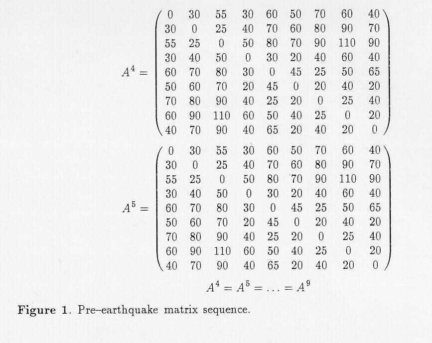