
SOLSTICE:  AN ELECTRONIC JOURNAL OF GEOGRAPHY AND MATHEMATICS

http://www.imagenet.org

WINTER, 1999

VOLUME X, NUMBER 2

ANN ARBOR, MICHIGAN


Founding Editor-in-Chief:
     Sandra Lach Arlinghaus, University of Michigan;
        Institute of Mathematical Geography (independent)

Editorial Advisory Board:
  Geography.
     Michael F. Goodchild, University of California, Santa Barbara
     Daniel A. Griffith, Syracuse University
     Jonathan D. Mayer, University of Washington (also School of Medicine)
     John D. Nystuen, University of Michigan
  Mathematics.
     William C. Arlinghaus, Lawrence Technological University
     Neal Brand, University of North Texas
     Kenneth H. Rosen, A. T. & T. Bell Laboratories
  Engineering Applications.
     William D. Drake, University of Michigan
  Education.
     Frederick L. Goodman, University of Michigan
  Business.
     Robert F. Austin, Austin Communications Education Services.

Book Review Editors:
     Richard Wallace, University of Michigan.
     Kameshwari Pothukuchi, Wayne State University

Web Design:
     Sandra L. Arlinghaus
     (with early input from William E. Arlinghaus).

WebSite:  http://www.imagenet.org

Electronic address:  sarhaus@umich.edu


MISSION STATEMENT

     The purpose of Solstice is to promote interaction between geography

and mathematics. Articles in which elements of one discipline are used to

shed light on the other are particularly sought.  Also welcome are

original contributions that are purely geographical or purely

mathematical.  These may be prefaced (by editor or author) with commentary

suggesting directions that might lead toward the desired interactions.

Individuals wishing to submit articles or other material should contact an

editor, or send e-mail directly to sarhaus@umich.edu.


SOLSTICE ARCHIVES

     Back issues of Solstice are available on the WebSite of the Institute

of Mathematical Geography, http://www.imagenet.org and at various sites

that can be found by searching under "Solstice" on the World Wide Web.

Thanks to Bruce Long (Arizona State University, Department of Mathematics)

for taking an early initiative in archiving Solstice using GOPHER.


PUBLICATION INFORMATION

     The electronic files are issued yearly as copyrighted hardcopy in the

Monograph Series of the Institute of Mathematical Geography.  This

material will appear in a Volume in that series, ISBN to be announced.

To order hardcopy, and to obtain current price lists, write to the

Editor-in-Chief of Solstice at 1964 Boulder Drive, Ann Arbor, MI 48104, or

call 734-975-0246.

     Suggested form for citation:  cite the hardcopy.  To cite the

electronic copy, note the exact time of transmission from Ann Arbor, and

cite all the transmission matter as facts of publication.  Any copy that

does not superimpose precisely upon the original as transmitted from Ann

Arbor should be presumed to be an altered, bogus copy of Solstice.  The

oriental rug, with errors, serves as the model for creating this weaving

of words and graphics.
EMail from Readers.
This past month IMaGe has received four notes of the same content, all having to do with the astronomical winter solstice of 1999. We reprint the material, forwarded by:
Robert F. Austin
John D. Nystuen
James R. O'Neil
Sandra S. Westrin
in the table below.
| "This year will be the first full moon to occur on the winter solstice [in 133 years], Dec. 22, commonly called the first day of winter. Since a full moon on the winter solstice occurs in conjunction with a lunar perigee (point in the moon's orbit that is closest to Earth) the moon will appear about 14% larger than it does at apogee (the point in its elliptical orbit that is farthest from the Earth). Since the Earth is also several million miles closer to the sun at this time of the year than in the summer, sunlight striking the moon is about 7% stronger, making it brighter. Also, this will be the closest perigee of the moon of the year since the moon's orbit is constantly deforming. If the weather is clear and there is snow cover where you live, it is believed that even car headlights will be superfluous. On December 21st, 1866 the Lakota Sioux took advantage of this combination of occurrences and staged a devastating retaliatory ambush on soldiers in the Wyoming Territory. In laymen's terms all this means it will be a super bright full moon, much more than the usual AND it hasn't happened this way for 133 years! Our ancestors 133 years ago saw this. It will be 100 years or so years from now until our descendants will see this again." |
for John D. Nystuen Career Commemorative Symposium, held in Ann
Arbor,
September 24, 1999, at the Pendleton Room of the Michigan Union has
been
produced. People who attended the symposium will be receiving a
CD
in the mail. Other interested parties, should feel free to
contact
John Nystuen concerning it (nystuen@umich.edu) with a copy of the
e-mail
note to IMaGe (sarhaus@umich.edu).
Jeffrey A. Nystuen
Senior Oceanographer
University of Washington
presented at
The John D. Nystuen Symposium
The University of Michigan
Ann Arbor, Michigan
24 September 1999
Abstract: The sound of rain underwater is loud and distinctive. It can be used as a signal to detect and measure oceanic rainfall. These measurements are needed to support climatological studies of the distribution and intensity of global rainfall patterns. Individual raindrops produce sound underwater by their impacts onto the ocean surface and, more importantly, by sound radiation from any bubbles trapped underwater during their splashes. Because different raindrop sizes produce distinctive sounds, the underwater sound can be inverted to quantitatively measure drop size distribution in the rain. Acoustical Rain Gauges (ARGs) are being deployed on oceanic moorings to make long-term measurements of rainfall using this acoustical technique.
1. Why listen to raindrops?
Rain is one of the most important components of climate. Knowledge of its distribution and intensity is important not only to farmers and flood control planners, but also to meteorologists, oceanographers and climatologists. This is because the formation of a raindrop in the air is accompanied by latent heat release. This heat release is one of the primary sources of energy driving atmospheric circulation. Thus, understanding the global patterns of distribution and intensity of rainfall is needed to improve weather and climate forecasting. Furthermore layers of relatively fresh water due to rain at the ocean surface are now thought to significantly affect oceanic circulation1, another component of global climate. Unfortunately, rainfall is also very difficult to measure, especially over the ocean where few people live and where rain gauges commonly used on land don't work. But we all know that rain falling onto a tin roof makes a lot of noise, and so does rain falling onto water. In fact, rain falling onto water is one of the loudest sources of underwater sound. So maybe we can measure oceanic rain by listening to it from below the ocean surface.
2. How do raindrops make sound underwater?
There are actually two components to the sound generated by a raindrop splash. These are the splat (impact) of the drop onto the water surface and then the subsequent formation of a bubble underwater during the splash. The relative importance of these two components of sound depends on the raindrop size. Surprisingly, for most raindrops, it is the bubble that is, by far, the loudest sound source. Bubbles are one of the most important components of underwater sound2. They have two stages during their lifetimes: screaming infant bubbles and quiet adult bubbles. As a bubble is created, in general it is not in equilibrium with its environment. It radiates sound (screams) to reach equilibrium. The frequency of the sound is well defined3:

and depends on bubble radius, a, local pressure, P0, local water density, r 0, and a geophysical constant, g = 1.4. The important observation is that the size of the bubble is inversely proportional to its resonance (ringing) frequency. Larger bubbles ring at lower frequencies. The sound radiated is often loud and narrowly tuned in frequency (a pure tone). But quickly, after just tens of milliseconds, a bubble in water becomes a quiet adult bubble and changes roles. It absorbs sound, and is especially efficient absorbing sound at its resonance frequency.
Naturally occurring raindrops range in size from about 300 microns diameter (a drizzle droplet) to over 5 mm diameter (often at the beginning of a heavy downpour). As the drop size changes, the shape of the splash changes and so does the subsequent sound production. Laboratory and field studies4,5 have been used to identify five acoustic raindrop sizes (Table 1). For tiny drops (diameter < 0.8 mm), the splash is gentle, and no sound is detected. On the other hand, small raindrops (0.8 - 1.2 mm diameter) are remarkably loud. The impact component of their splash is still very quiet, but the geometry of the splash is such that a bubble is generated by every splash in a very predictable manner6. These bubbles are relatively uniform in size, and therefore frequency, and are very loud underwater. Small raindrops are present in almost all types of rainfall, including light drizzle, and are therefore responsible for the remarkably loud and unique underwater "sound of drizzle" heard between 13-25 kHz, the resonance frequency for these bubbles.
TABLE 1. Acoustic raindrop sizes. The raindrop
sizes
are identified by different physical mechanisms associated with the
drop
splashes (4, 5).
| Drop size | Diameter | Sound source | Frequency range | Splash character |
| tiny | <0.8 mm | silent | a | gentle |
| small | 0.8-1.2 mm | loud bubble | 13-25 kHz | gentle, with bubble every splash |
| medium | 1.2-2.0 mm | weak impact | 1-30 kHz | gentle, no bubbles |
| large | 2.0-3.5 mm | impact
loud bubbles |
1-35 kHz
2-35 kHz |
turbulent
irregular bubble entrainment |
| very large | >3.5 mm | loud impact
loud bubbles |
1-50 kHz
1-50 kHz |
turbulent
irregular bubble entrainment penetrating jet |
Interestingly, the splash of the next larger raindrop size, medium (1.2-2.0 mm diameter), does not trap bubbles underwater, and consequently medium raindrops are relatively quiet, much quieter than the small raindrops. The only acoustic signal from these drops is a weak impact sound spread over a wide frequency band. For large (2.0-3.5 mm diameter) and very large (> 3.5 mm) raindrops, the splash becomes energetic enough that a wide range of bubble sizes are trapped underwater during the splash, producing a loud sound that includes relatively low frequencies (1 - 10 kHz) from the larger bubbles. For very large raindrops, the splat of the impact is also very loud with the sound spread over a wide frequency range (1-50 kHz). Thus, each drop size produces sound underwater with unique spectral features that can be used to acoustically identify the present of that drop size within the rain.
An example of the underwater sound field generated by a heavy thunderstorm recorded in Miami, FL is shown in Figure 1. The variations in the sound field are associated with changes in the drop size distribution (Fig. 2). During the heavy convective downpour, with rainfall rates reaching 150 mm/hr, very large raindrops are present and the sound field is loud across the entire spectrum (1-50 kHz). At the end of the convective downpour, a long drizzle begins. This phase of the storm has few large drops. The sound generated by small drops dominates the sound field producing the distinctive 13-25 kHz peak in the sound field associated with drizzle. At the end of the event, a few large drops are again present and once again the sound field becomes elevated below 10 kHz. Because the sound signatures for each drop size are unique, it is possible to invert the underwater sound field to acoustically estimate the drop size distribution within the rain5 (Fig. 2). Once an acoustic drop size distribution is obtained, a variety of interesting features associated with the rain can be calculated, for example, rainfall rate or median drop size.

Figure 1. The underwater sound field during a thunderstorm. The changes in the sound are closely associatied with changes in the drop size distribution of the rain.

Figure 2. The observed drop size distribution in the thunderstorm and the acoustical inversion based on the unique sound signatures for each drop size. Very large raindrops are present during the heavy downpour. During the following drizzle, only small and medium raindrops are present and the sound of drizzle is heard between 13-25 kHz. Still later, a few large raindrops are present and the sound levels below 10 kHz become higher once again.
3. Listening to the Ocean: Acoustic Rain Gauges
In order to measure rain at sea, Acoustic Rain Gauges (ARGs) have
been
designed and built at the Applied Physics Laboratory, University of
Washington.
The ARG consists of a hydrophone (underwater microphone), some
electronic
circuitry, a low-power sampling computer and a battery package designed
to operate the ARG without servicing for up to a year. The ARG is
attached
to a mooring line, and can be placed at any depth, although practically
the depth is limited by the crushing strength of the instrument case.
Every
few minutes the ARG "wakes up", evaluates and records the underwater
sound
field. Currently, the ARG design is autonomous from the surface float,
and the recovery of data awaits recovery of the mooring. In the future,
real-time transmission of the data will be needed to provide useful
data
for weather forecasting.

Figure 3. Dr. Jeffrey A. Nystuen holding an Acoustic Rain Gauge (ARG). This instrument is designed to be clamped onto an oceanic mooring and will record the underwater sound for one year.
4. Detection and Measurement of Rain at Sea
When listening for rain in the ocean, the first step is to identify the sound as rain. There are lots of other sounds underwater, including the sounds of waves breaking, man-made sounds and biological sounds. Biological and man-made sounds are sometimes very loud and, if they contain frequency components which overlap the rain-generated sound, then they can prevent acoustical measurement of rain. These noises are usually intermittent or geographically localized. Some locations where persistent "noise" is present includes harbors (shipping and industrial activity) and snapping shrimp colonies. Snapping shrimp are from a family of shrimp species which make very loud "snaps" and that inhabit shallow tropical waters. Fortunately, the frequency content of most sounds is unique to their sources, and can be used to identify the sources, including rain, drizzle and whitecaps. Some examples of oceanic sound spectra are shown in Fig. 4.

Figure 4. Examples of underwater sound spectra
recorded
from an oceanic mooring in the South China Sea. The sound spectra from
wind-only conditions (cyan) show an uniform shape and a sound level
which
is proportional to wind speed. The sound of drizzle (green) shows the
characteristic
peak associated with the sound generation mechanism of the small
raindrops.
The sound of heavy rain (red) is louder and includes lower frequencies.
The sound of extreme rain includes sound generated by very large
raindrops
and is very loud. It also shows the effect of "quiet adult bubbles".
Two
spectra from extreme rain (200 mm/hr) are shown. The first (red) shows
extremely high sound levels at all frequencies. The second (magenta)
shows
relatively lower sound levels above 10 kHz. This spectrum was recorded
five minutes after the first, and yet the rainfall rate was still the
same.
A layer of bubbles had been injected into the sea surface. New "rain
sound"
has to pass through the bubble layer to reach the ARG sensor, and is
partially
absorbed by the bubbles. Since smaller bubbles (higher resonance
frequency)
are less buoyant than larger bubbles, they stay in the water longer and
thus, this bubble effect is most noticable at higher frequencies.

Figure 5. Acoustic weather classification uses features of the underwater sound spectrum to identify the sound source: wind (cyan), drizzle (green), rain (red), extreme rain (magenta) and to detect ambient bubbles.

Figure 6. A temporal history of the sound
field
over three days at four different frequencies from the North Atlantic
Ocean
(ASREX Experiment, sponsored by Office of Naval Research). The lowest
frequency
(500 Hz) is not affected by precipitation, while the highest frequency
(20 kHz) is affected by rain, drizzle and ambient bubbles. The acoustic
interpretation of the sound record measures wind speed (cyan), rainfall
rate (red) and detects drizzle (green). Comparison data for wind speed
(blue) and near-surface salinity (magenta) from a nearby surface
mooring
are also shown.
5. Conclusions
The sound of rain underwater is a loud and distinctive signal which can be used to detect and measure rain at sea. Individual raindrops make sound underwater by two distinct mechanisms: the impact of the raindrop onto the ocean surface and sound radiation from any bubbles trapped underwater during the splash. For most raindrops, the sound radiation by bubbles is, by far, the louder sound source. Because the geometry of their splashes regularly trap a bubble of uniform size, small raindrops (0.8-1.2 mm diameter) are unexpectedly loud underwater. These drops are responsible for the remarkably loud "sound of drizzle" heard between 13-25 kHz. Medium raindrops (1.2-2.0 mm diameter) are relatively quiet, while large (2.0-3.5 mm diameter) and very large (> 3.5 mm) raindrops have energetic splashes which can trap larger bubbles. These bubbles radiate sound at frequencies as low as 1 kHz. Because the different raindrop sizes produce sound with distinctive features, the sound field can be "inverted" to measure the raindrop size distribution within the rain. This is a good measure of rainfall rate, or other interesting features of rainfall.
Although there are sometimes man-made or biological noises which are loud and could potentially interfere with the acoustical measurement of rain, these noises are generally intermittent or geographically localized. When rain is present, the sound from rain dominates the underwater sound field. There are two features of rain and drizzle generated sound that allow detection of rain at sea. These are the relative level (very loud) and the relatively higher sound levels at higher frequency (over 10 kHz) when compared to wind. By monitoring for these distinctive spectral features, it is possible to detect and then quantify rainfall at sea.
New ARGs are currently being deployed on several of the moorings that form the Tropical Atmosphere Ocean (TAO) deep ocean mooring array deployed by NOAA in the tropical Pacific Ocean13. Data from these ARGs should become available for scientists beginning in the year 2000. By learning to listen to the ocean we can make important rainfall observations which will help meteorologists, oceanographers and climatologists to better understand the distribution and intensity of this important component of climate.
6. Acknowledgments
My father, Prof. John D. Nystuen, has had a pervasive and yet non-specific influence on my career. He inspired me to pursue an academic career. My most influential scientific colleague has been Prof. Herman Medwin from the Naval Postgraduate School, Monterey, California. Other key colleagues include my graduate and post-graduate advisors, Profs. Robert Stewart, Walter Munk and Dr. David Farmer. Long-term funding for my research has been from the Office of Naval Research - Ocean Acoustics (ONR Code OA321), but also from the National Science Foundation (NSF), the National Oceanic and Atmospheric Administration - Pan-American Climate Studies (NOAA-PACS) and, most recently, the National Aeronautics and Space Administration - Tropical Rain Measuring Mission (NASA-TRMM).
7. References
1. S.P. Anderson, S.P., R.A.Weller and R. Lukas, 1996: Surface buoyancy forcing and the mixed layer of the western Pacific warm pool: Observations and 1-D model results. J Climate 9, 3056-3085.
2. C.S. Clay and H. Medwin, 1977, Acoustical Oceanography, Chapter 6, Wiley, New York, 544p.
3. M. Minnaert, 1933: On musical air bubbles and the sounds of running water. Philos. Mag. 16, 235-248.
4. H. Medwin, J.A. Nystuen, P.W. Jacobus, L.H. Ostwald and D.E. Synder, 1992: The anatomy of underwater rain noise. J. Acoust. Soc. Am. 92, 1613-1623.
5 .J.A. Nystuen, 1996: Acoustical rainfall analysis: Rainfall drop size distribution using the underwater sound field. J. Acoust. Soc. Am. 13, 74-84.
6. H.C. Pumphrey, L.A. Crum and L. Bjorno, 1989: Underwater sound produced by individual drop impacts and rainfall. J. Acoust. Soc. Am. 85, 1518-1526.
7. S. Vagle, W.G. Large and D.M. Farmer, 1990: An evaluation of the WOTAN technique for inferring oceanic wind from underwater sound. J. Atmos. and Ocean. Tech. 7, 576-595.
8. H. Medwin and M.M. Beaky, 1989: Bubble sources of the Knudsen sea noise spectrum. J. Acoust. Soc. Am. 83, 1124-1130.
9. D.M. Farmer and D.D. Lemon, 1984: The influence of bubbles on the ambient noise in the ocean at high wind speeds. J. Phys. Oceanogr. 14, 1762-1778.
10. J.A. Nystuen and D.M. Farmer, 1989: Precipitation in the Canadian Atlantic Storms Program: Measurements of the Acoustic Signature. Atmosphere-Ocean27, 237-257.
11. J.A. Nystuen and H.D. Selsor, 1997: Weather classification using passive acoustic drifters. J. Atmos. and Oceanic Tech., 14, 656-666.
12. J.A. Nystuen, M.J. McPhaden and H.P. Freitag 1999: Surface Measurements of Precipitation from an Ocean Mooring: The Underwater Acoustic Log from the South China Sea", submitted to J. Applied Meteor.
13. M.J. McPhaden, A.J. Busalacchi, R. Cheney,
J.R.
Donguy, K.S. Gage, D. Halpern, M. Ji, P. Julian, G. Meyers, G.T.
Mitchum,
P.P. Niiler, J. Picaut, R.W. Reynolds, N. Smith and K. Takeuchi, 1998:
The Tropical Ocean-Global Atmosphere (TOGA) observing system: A decade
of progress. J. Geophys. Res, 103, 14,169-14,240.
Sandra Lach Arlinghaus
University of Michigan, School of Natural Resources and Environment
Community Systems Foundation
Institute of Mathematical Geography
The Environmental Protection Agency (EPA) maintains an online mapping facility, called Landview III, that contains data and site locations for hazardous sites of various sorts, as well as selected Census, United States Geological Survey, and other, data and boundary files. The user visits the EPA site and is permitted to download, free, the Landview software and one county boundary file and one county data file (per transmission). For those, such as precollegiate teachers, this is a marvelous resource for gaining some mini-GIS mapping capability. For those with full GISs on their desks, Landview also serves as a fine source of location and data files. The data files come in .dbf format and many already contain positional information as decimal degrees of latitude and longitude. Thus the files map easily in, for example, ArcView 3.2 (Environmental Systems Research Institute--ESRI). Simply open the table of interest and open that as an Event Theme which can then be converted to a shape file. The maps below offer an example of this capability. In addition to Landview III, other software packages used were: ArcView 3.2 (ESRI), Spatial Analyst Extension (ESRI), 3D Analyst Extension (ESRI), Animal Movement Extension to ArcView (free), Adobe PhotoShop 5.5, Netscape Communicator 4.05, and MS Excel (Microsoft Office 97, Professional version) Windows 98 (Microsoft).
 |
Map 2. A natural next step in the mapping process might
be to create a thematic map using Census data for the
blockgroups.
One might consider demographics of various sorts in relation to EPA
site
location. The map below shows the blockgroup polygons colored by
racial categories of "black" or African-American population and "white"
or Caucasian-American population normalized by 1990 total population
for
each blockgroup. Deeper shades of purple indicate higher
densities
of African-American population. One direction that further
mapping
effort might take is to overlay other boundary files, such as rivers,
and
also to create more thematic maps based on other demographic, economic,
and physical variables. The remaining maps suggest another
approach.
 |
Map 3. The blockgroup boundaries were removed. A
grid of points, spaced at 0.01 degrees of latitude and longitude was
superimposed
on the map. The grid database was created in Excel and brought
into
ArcView as an Event Theme.
 |
Map 4. The grid points were assigned weights based on
distance
from EPA sites. Those points closest were colored with the
darkest
shade of red; those fartheset away with the lightest shade. The
distances
were calculated in Animal Movement Extension (Hooge and Eichenlaub,
1997),
Movement|Calculate Distance, with distances measured from EPA sites to
grid points. These distances were then used as weights and the
grid
points (as a shape file) were shaded using a standard color ramp.
Weights might be assigned using any of a number of standard weighting
techniques
or using technique designed by the cartographer or other map creator
(Tobler
and Wineberg, c.1975 is one classic example).
 |
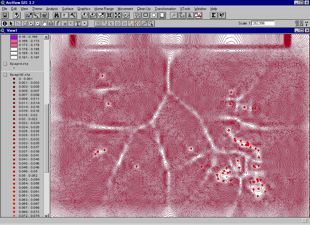
Map 5. The grid points were then finely contoured, in
0.001
parts of a unit. The Surface|Create Contours command was
employed.
The method of interpolation chosen was Spline, the Z-value used was the
distance value calculated above, and the type of contour selected was a
tension contour. Here the screen capture is placed directly from
ArcView into the html file. Note the apparent swale
lines
and saddle points in the contouring representing troughs based on the
distance
data and peaks or flat surface surrounding the actual sites.
 |
Map 6. The contours were then converted to a
Triangulated
Irregular Network (TIN) (Arlinghaus et al., 1994) to suggest a surface
based on distance from EPA sites. Warm colors represent locations
close to numerous EPA sites; cool colors represent locations farthest
from
EPA sites. Shading, coupled with the use of a finely-contoured
surface,
make the peaks and valleys stand out. The TIN is calculated by
the
software; basically, it triangulates the contours creating tiny
triangular
facets, which when colored and shaded, suggest a surface.
 |
Map 7. The TIN is then covered with the thematic map
shown
in Map 2. Here, once again, the demographic data is calculated by
block group: percent "black" and percent "white". Denser
patterns
of black and white represent greater block group densities of
African-American
and Caucasian-American populations. The block group boundaries
were
colored transparent as were the backgrounds behind the patterns so that
the TIN would show through. To preserve the invisible background
outside of ArcView, the Windows-universal screen capture,
Alt+PrintScreen,
was used to put a copy of the screen image on the Windows
Clipboard.
The clipboard was then pasted (Ctrl+v) into a blank canvas (File|New)
in
Adobe PhotoShop (which senses the size of the Clipboard image on
opening
a new blank canvas) where the image was cropped.
 |
The evidence of maps can communicate information differently to
different
people. As mapping software becomes easier and easier to use, one
can only hope that curricular matters keep pace. Maps like these
in the hands of a policy maker can be helpful or dangerous weapons;
fine
geographic education can make them become the former.
Arlinghaus, S. Austin, R., Arlinghaus, W., Drake, W., and Nystuen, J. Practical Handbook of Digital Mapping Terms and Concepts. CRC Press. 1994.
Hooge, P. N. and B. Eichenlaub. 1997. Animal movement extension to ArcView. ver. 1.1 and later. Alaska Biological Science Center, U.S. Geological Survey, Anchorage, AK, USA.
Tobler, W. R. and Wineberg, S. c.1975. A Cappadocian
speculation.
Nature.
Quotation from the back cover appears in the table below:
| "New practical techniques for nonlinear system research
and evaluation
Nonlinear Systems Techniques and Applications provides the most practical techniques currently available for analyzing and identifying nonlinear systems from random data measured at the input and output points of the nonlinear systems. These new techniques require only one-dimensional spectral functions that are much simpler to compute and apply than previous nonlinear procedures. The new results show when and how to replace a wide class of single input/single-output nonlinear models with simpler equivalent multiple-input/single-output linear models. While other techniques are usually restricted to Gaussian data, the new techniques developed here apply to data with arbitrary probability, correlation, and spectral properties. Numerous examples used in the book are based on the analysis of real physical data passing through real nonlinear systems in the fields of oceanography, automotive engineering, and biomedical research. For practicing engineers and scientists involved in aerospace,
automotive,
biomedical, electrical, mechanical, oceanographic, and other activities
concerned with nonlinear system analysis, Nonlinear Systems
Techniques
and Applications is the essential reference work in the field."
|